9 The Normal Random Variable

9.1 Student Learning Objective

This chapter introduces a very important bell-shaped distribution known as the Normal distribution. Computations associated with this distribution are discussed, including the percentiles of the distribution and the identification of intervals of subscribed probability. The Normal distribution may serve as an approximation to other distributions. We demonstrate this property by showing that under appropriate conditions the Binomial distribution can be approximated by the Normal distribution. This property of the Normal distribution will be picked up in the next chapter where the mathematical theory that establishes the Normal approximation is demonstrated. By the end of this chapter, the student should be able to:

• Understand the pnorm and qnorm functions

• Recognize the Normal density and apply R functions for computing Normal probabilities and percentiles.

• Associate the distribution of a Normal random variable with that of its standardized counterpart, which is obtained by centering and re-scaling.

• Use the Normal distribution to approximate the Binomial distribution.

9.2 The Normal Random Variable

The Normal distribution is the most important of all distributions that are used in statistics. In many cases it serves as a generic model for the distribution of a measurement. Moreover, even in cases where the measurement is modeled by other distributions (i.e. Binomial, Poisson, Uniform, Exponential, etc.) the Normal distribution emerges as an approximation of the distribution of numerical characteristics of the data produced by such measurements.

9.2.1 The Normal Distribution

A Normal random variable has a continuous distribution over the sample space of all numbers, negative or positive. We denote the Normal distribution via \(Y \sim \mathrm{Normal}(\mu, \sigma)\), where \(\mu = \operatorname{E}(Y)\) is the expectation of the random variable and \(\sigma = \sqrt{\operatorname{Var}(Y)}\) is it’s standard deviation⁵⁵.

Consider, for example, \(Y \sim \mathrm{Normal}(\mu=2,\sigma=3)\). The density of the distribution is presented in Figure 9.1. Observe that the distribution is symmetric about the expectation 2. The random variable is more likely to obtain its value in the vicinity of the expectation. Values much larger or much smaller than the expectation are substantially less likely.

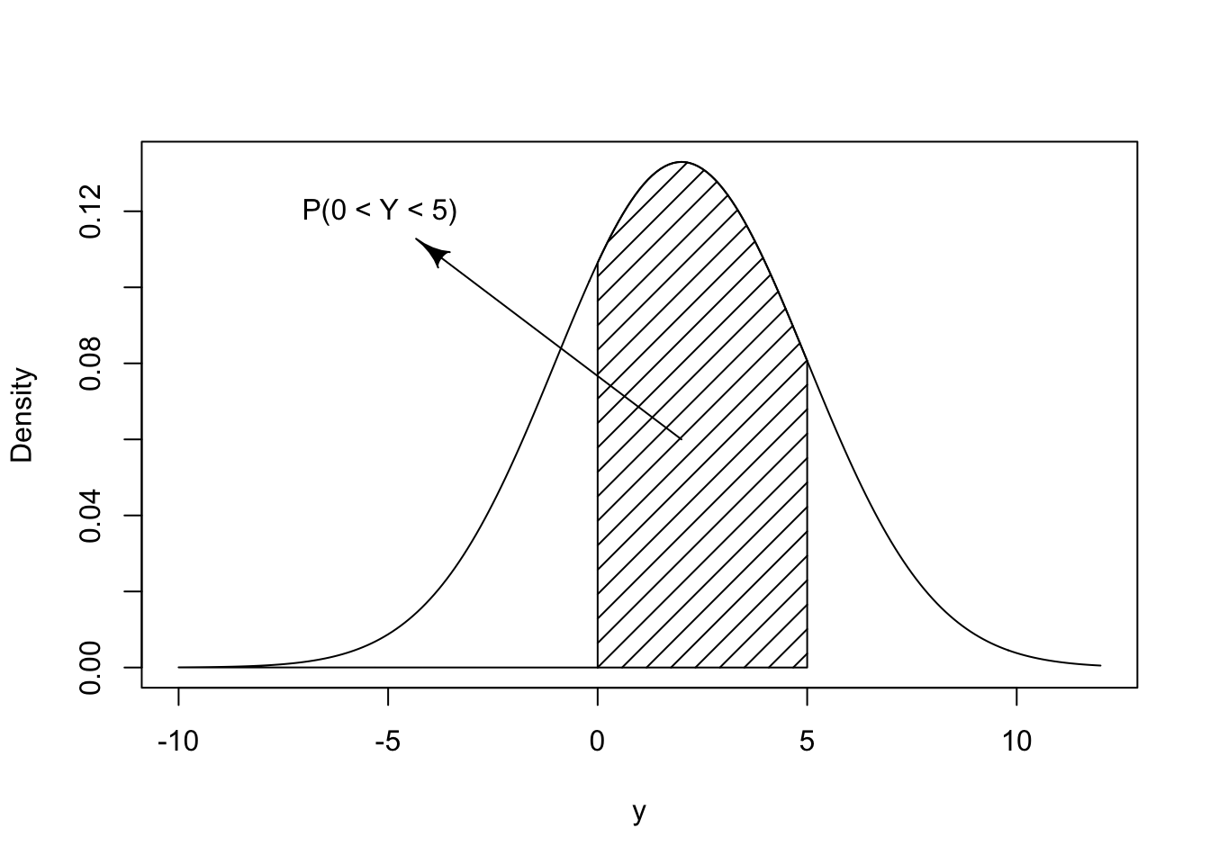
Figure 9.1: The Normal(2,3) Distribution

The density of the Normal distribution can be computed with the aid of the function dnorm. The cumulative probability can be computed with the function pnorm. For illustrating the use of the latter function, assume that \(Y \sim \mathrm{Normal}(2,3)\). Say one is interested in the computation of the probability \(\operatorname{P}(0 < Y \leq 5)\) that the random variable obtains a value that belongs to the interval \((0,5]\). The required probability is indicated by the marked area in Figure 9.1. This area can be computed as the difference between the probability \(\operatorname{P}(Y \leq 5)\), the area to the left of 5, and the probability \(\operatorname{P}(Y \leq 0)\), the area to the left of 0:

pnorm(q = 5, mean = 2, sd = 3) - pnorm(q = 0, mean = 2, sd = 3)
#> [1] 0.5888522

The difference is the indicated area that corresponds to the probability of being inside the interval, which turns out to be approximately equal to 0.589. Notice that the expectation \(\mu\) of the Normal distribution is entered as the second argument to the function. The third argument to the function is the standard deviation, i.e. the square root of the variance.

We can alternatively use the mosaic R package to compute this probability, which also outputs a graph by default:

mosaic::xpnorm(q = c(0,5), mean = 2, sd = 3)

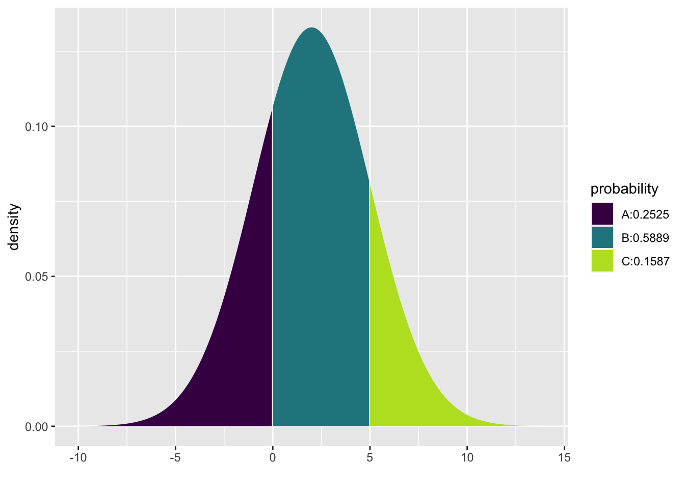
#> [1] 0.2524925 0.8413447

Figure 9.2 displays the densities of the Normal distribution for the combinations \(\mu= 0\), \(\sigma = 1\) (the red line); \(\mu = 2\), \(\sigma = 3\) (the black line); and \(\mu = -3\), \(\sigma = 1/2\) (the green line). Observe that the smaller the variance the more concentrated is the distribution of the random variable about the expectation.

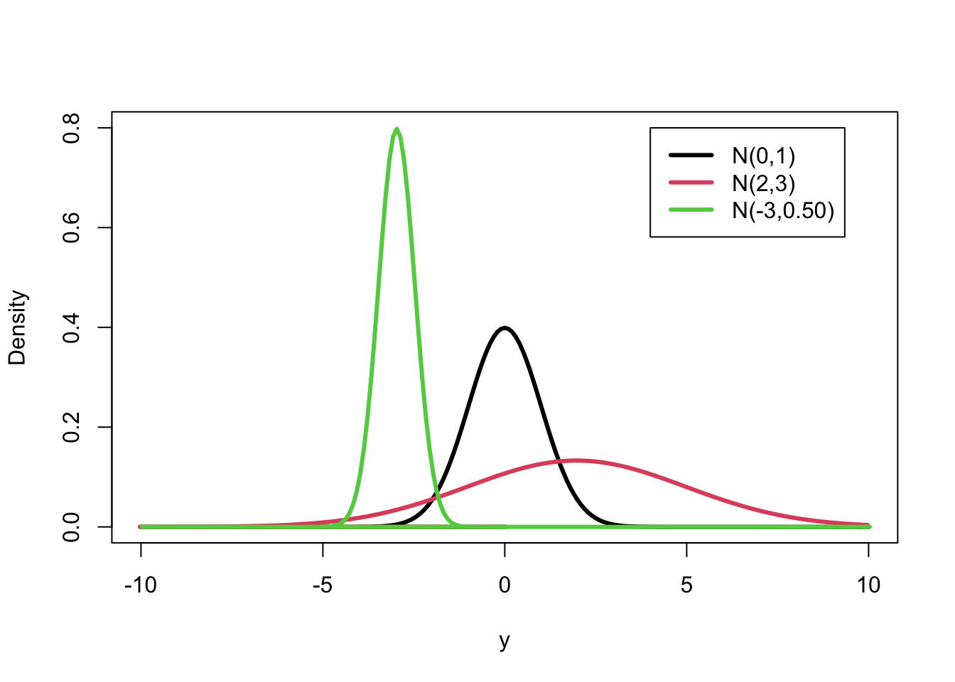
Figure 9.2: The Normal Distribution for Various Values of \(\mu\) and \(\sigma\)

Example 9.1 IQ tests are a popular (and controversial) mean for measuring intelligence. They are produced as (weighted) average of a response to a long list of questions, designed to test different abilities. The score of the test across the entire population is set to be equal to 100 and the standard deviation is set to 15. The distribution of the score is Normal. Hence, if \(Y\) is the IQ score of a random subject then \(Y \sim \mathrm{Normal}(100,15)\).

Example 9.2 Any measurement that is produced as a result of the combination of many independent influencing factors is likely to poses the Normal distribution. For example, the hight of a person is influenced both by genetics and by the environment in which that person grew up. Both the genetic and the environmental influences are a combination of many factors. Thereby, it should not come as a surprise that the heights of people in a population tend to follow the Normal distribution.

9.2.2 The Standard Normal Distribution

The standard normal distribution is a normal distribution of standardized values, which are called \(z\)-scores. A \(z\)-score is the original measurement measured in units of the standard deviation from the expectation. For example, if the expectation of a Normal distribution is 2 and the standard deviation is \(3 = \sqrt{9}\), then the value of 0 is 2/3 standard deviations smaller than (or to the left of) the expectation. Hence, the \(z\)-score of the value 0 is -2/3.

The standard Normal distribution is the distribution of a standardized Normal measurement. The expectation for the standard Normal distribution is 0 and the variance is 1. When \(Y \sim N(\mu,\sigma)\) has a Normal distribution with expectation \(\mu\) and standard deviation \(\sigma\) then the transformed random variable \(Z = (Y-\mu)/\sigma\) produces the standard Normal distribution \(Z\sim N(0,1)\). The transformation corresponds to the re-expression of the original measurement in terms of a new “zero” and a new unit of measurement. The new “zero” is the expectation of the original measurement and the new unit is the standard deviation of the original measurement.

Computation of probabilities associated with a Normal random variable \(Y\) can be carried out with the aid of the standard Normal distribution. For example, consider the computation of the probability \(\operatorname{P}(0 < Y \leq 5)\) for \(Y \sim N(2, 3)\), that has expectation \(\mu=2\) and standard deviation \(\sigma = 3\). Consider \(Y\)’s standardized values: \(Z = (Y-2)/3\). The boundaries of the interval \([0,5]\), namely \(0\) and \(5\), have standardized \(z\)-scores of \((0-2)/3=-2/3\) and \((5-2)/3 =1\), respectively. Clearly, the original measurement \(Y\) falls between the original boundaries (\(0 < Y \leq 5\)) if, and only if, the standardized measurement \(Z\) falls between the standardized boundaries (\(-2/3 < Z \leq 1\)). Therefore, the probability that \(Y\) obtains a value in the range \([0,5]\) is equal to the probability that \(Y\) obtains a value in the range \([-2/3,1]\).

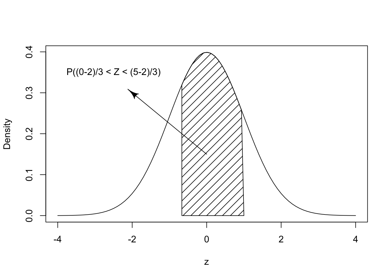
Figure 9.3: The Standard Normal Distribution

The function “pnorm” was used in the previous subsection in order to compute that probability that \(X\) obtains values between 0 and 5. The computation produced the probability 0.5888522. We can repeat the computation by the application of the same function to the standardized values:

pnorm(q = (5-2)/3) - pnorm(q = (0-2)/3)
#> [1] 0.5888522

The value that is being computed, the area under the graph for the standard Normal distribution, is presented in Figure 9.3. Recall that 3 arguments where specified in the previous application of the function pnorm: the \(x\) value, the expectation, and the standard deviation. In the given application we did not specify the last two arguments, only the first one. (Notice that the output of the expression (5-2)/3 is a single number and, likewise, the output of the expression (0-2)/3 is also a single number.) Most R function have many arguments that enables flexible application in a wide range of settings. For convenience, however, default values are set to most of these arguments. These default values are used unless an alternative value for the argument is set when the function is called. The default value of the second argument of the function pnorm that specifies the expectation is mean=0, and the default value of the third argument that specifies the standard deviation is sd=1. Therefore, if no other value is set for these arguments the function computes the cumulative distribution function of the standard Normal distribution.

9.2.3 Computing Percentiles

Consider the issue of determining the range that contains 95% of the probability for a Normal random variable. We start with the standard Normal distribution. Consult Figure 9.4. The figure displays the standard Normal distribution with the central region shaded. The area of the shaded region is 0.95.

We may find the \(z\)-values of the boundaries of the region, denoted in the figure as \(z_0\) and \(z_1\) by the investigation of the cumulative distribution function. Indeed, in order to have 95% of the distribution in the central region one should leave out 2.5% of the distribution in each of the two tails. That is, 0.025 should be the area of the unshaded region to the right of \(z_1\) and, likewise, 0.025 should be the area of the unshaded region to the left of \(z_0\). In other words, the cumulative probability up to \(z_0\) should be 0.025 and the cumulative distribution up to \(z_1\) should be 0.975.

In general, given a random variable \(Y\) and given a percent \(p\), the \(y\) value with the property that the cumulative distribution up to \(y\) is equal to the probability \(p\) is called the \(p\)-percentile of the distribution. Here we seek the 2.5%-percentile and the 97.5%-percentile of the standard Normal distribution.

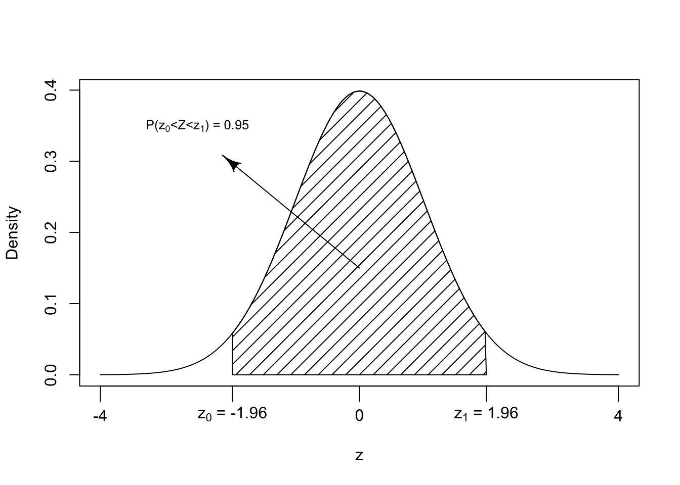
Figure 9.4: Central 95\(\%\) of the Standard Normal Distribution

The percentiles of the Normal distribution are computed by the function qnorm. The first argument to the function is a probability (or a sequence of probabilities), the second and third arguments are the expectation and the standard deviations of the normal distribution. The default values to these arguments are set to 0 and 1, respectively. Hence if these arguments are not provided the function computes the percentiles of the standard Normal distribution. Let us apply the function in order to compute \(z_1\) and \(z_0\):

qnorm(0.975)
#> [1] 1.959964
qnorm(0.025)
#> [1] -1.959964

Observe that \(z_1\) is practically equal to 1.96 and \(z_0 = -1.96 = -z_1\). The fact that \(z_0\) is the negative of \(z_1\) results from the symmetry of the standard Normal distribution about 0. As a conclusion we get that for the standard Normal distribution 95% of the probability is concentrated in the range \([-1.96, 1.96]\).

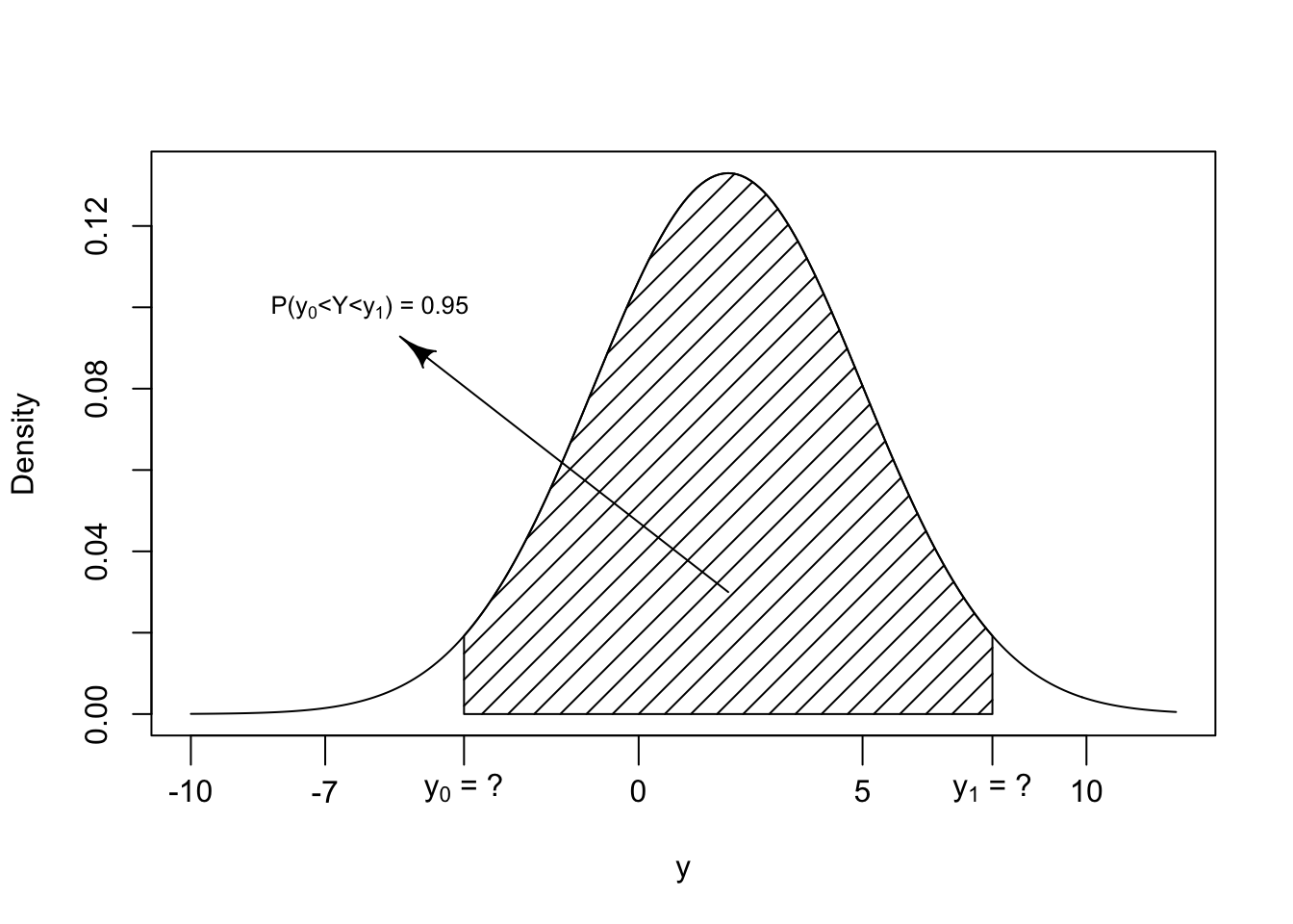
Figure 9.5: Central 95\(\%\) of the Normal(2,3) Distribution

The problem of determining the central range that contains 95% of the distribution can be addresses in the context of the original measurement \(Y\) (See Figure 9.5). We seek in this case an interval centered at the expectation 2, which is the center of the distribution of \(Y\), unlike 0 which was the center of the standardized values \(Z\). One way of solving the problem is via the application of the function qnorm with the appropriate values for the expectation and the standard deviation:

qnorm(0.975,2,3)
#> [1] 7.879892
qnorm(0.025,2,3)
#> [1] -3.879892

Hence, we get that \(y_0 = -3.88\) has the property that the total probability to its left is 0.025 and \(y_1 = 7.88\) has the property that the total probability to its right is 0.025. The total probability in the range \([-3.88, 7.88]\) is 0.95.

An alternative approach for obtaining the given interval exploits the interval that was obtained for the standardized values. An interval \([-1.96,1.96]\) of standardized \(z\)-values corresponds to an interval \([2 - 1.96 \cdot 3, 2 + 1.96\cdot 3]\) of the original \(x\)-values:

2 + qnorm(0.975)*3
#> [1] 7.879892
2 + qnorm(0.025)*3
#> [1] -3.879892

Hence, we again produce the interval \([-3.88,7.88]\), the interval that was obtained before as the central interval that contains 95% of the distribution of the \(\mathrm{Normal}(2,3)\) random variable.

In general, if \(Y \sim N(\mu,\sigma)\) is a Normal random variable then the interval \([\mu - 1.96 \cdot \sigma, \mu + 1.96 \cdot \sigma]\) contains 95% of the distribution of the random variable. Frequently one uses the notation \(\mu \pm 1.96 \cdot \sigma\) to describe such an interval.

9.2.4 The p and q functions: a summary

The ‘p’ function tells us, for a given value of the characteristic, what proportion of the distribution lies to the left of this specified value.

The ‘q’ (or quantile) function tells us, for a given proportion p, what is the value of the characteristic such that that specified proportion p of the distribution lies to the left of this ‘q’ value.

In Figure 9.6, the values of the p function are shown on the vertical axis, in red, against the (in this case, equally-spaced) values of the characteristic, shown on the horizontal axis. You enter on the horizontal axis, and exit with an answer on the vertical axis.

The q function (in blue) goes into the opposite direction. You enter at some proportion on the vertical axis, and exit with a value of the characteristic (a quantile) on the horizontal axis. In our plot, the proportions on the vertical axis are equally-spaced. Percentiles and quartiles are a very specific sets of quantiles: they are obtained by finding the values that divide the distribution into 100 or into 4.

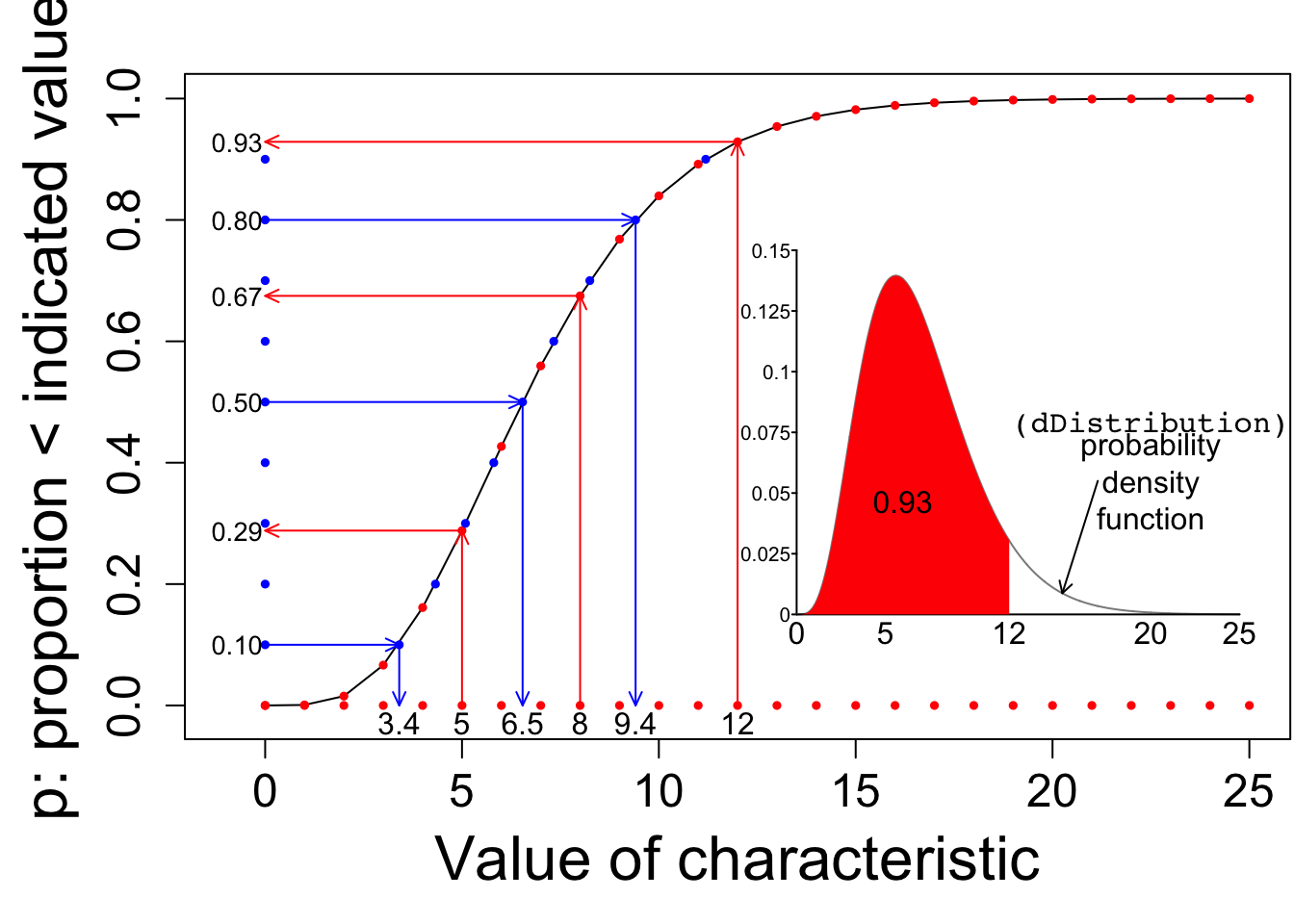
Figure 9.6: p and q functions visual representation.

9.2.5 Outliers and the Normal Distribution

Consider, next, the computation of the interquartile range in the Normal distribution. Recall that the interquartile range is the length of the central interval that contains 50% of the distribution. This interval starts at the first quartile (Q1), the value that splits the distribution so that 25% of the distribution is to the left of the value and 75% is to the right of it. The interval ends at the third quartile (Q3) where 75% of the distribution is to the left and 25% is to the right.

For the standard Normal the third and first quartiles can be computed with the aid of the function “qnorm”:

qnorm(0.75)
#> [1] 0.6744898
qnorm(0.25)
#> [1] -0.6744898

Observe that for the standard Normal distribution one has that 75% of the distribution is to the left of the value 0.6744898, which is the third quartile of this distribution. Likewise, 25% of the standard Normal distribution are to the left of the value -0.6744898, which is the first quartile. the interquartile range is the length of the interval between the third and the first quartiles. In the case of the standard Normal distribution this length is equal to \(0.6744898 - (-0.6744898) = 1.348980\).

We previously considered box plots as a mean for the graphical display of numerical data. The box plot includes a vertical rectangle that initiates at the first quartile and ends at the third quartile, with the median marked within the box. The rectangle contains 50% of the data. Whiskers extends from the ends of this rectangle to the smallest and to the largest data values that are not outliers. Outliers are values that lie outside of the normal range of the data. Outliers are identified as values that are more then 1.5 times the interquartile range away from the ends of the central rectangle. Hence, a value is an outlier if it is larger than the third quartile plus 1.5 times the interquartile range or if it is less than the first quartile minus 1.5 times the interquartile range.

How likely is it to obtain an outlier value when the measurement has the standard Normal distribution? We obtained that the third quartile of the standard Normal distribution is equal to 0.6744898 and the first quartile is minus this value. The interquartile range is the difference between the third and first quartiles. The upper and lower thresholds for the defining outliers are:

qnorm(0.75) + 1.5*(qnorm(0.75)-qnorm(0.25))
#> [1] 2.697959
qnorm(0.25) - 1.5*(qnorm(0.75)-qnorm(0.25))
#> [1] -2.697959

Hence, a value larger than 2.697959 or smaller than -2.697959 would be identified as an outlier.

The probability of being less than the upper threshold 2.697959 in the standard Normal distribution is computed with the expression “pnorm(2.697959)”. The probability of being above the threshold is 1 minus that probability, which is the outcome of the expression “1-pnorm(2.697959)”.

By the symmetry of the standard Normal distribution we get that the probability of being below the lower threshold -2.697959 is equal to the probability of being above the upper threshold. Consequently, the probability of obtaining an outlier is equal to twice the probability of being above the upper threshold:

2*(1-pnorm(2.697959))
#> [1] 0.006976603

We get that for the standard Normal distribution the probability of an outlier is approximately 0.7%.

9.3 Approximation of the Binomial Distribution

The Normal distribution emerges frequently as an approximation of the distribution of data characteristics. The probability theory that mathematically establishes such approximation is called the Central Limit Theorem and is the subject of subsequent chapters. In this section we demonstrate the Normal approximation in the context of the Binomial distribution.

9.3.1 Approximate Binomial Probabilities and Percentiles

Consider, for example, the probability of obtaining between 1940 and 2060 heads when tossing 4,000 fair coins. Let \(Y\) be the total number of heads. The tossing of a coin is a trial with two possible outcomes: “Head” and “Tail.” The probability of a “Head” is 0.5 and there are 4,000 trials. Let us call obtaining a “Head” in a trial a “Success”. Observe that the random variable \(Y\) counts the total number of successes. Hence, \(Y \sim \mathrm{Binomial}(4000,0.5)\).

The probability \(\operatorname{P}(1940 \leq Y \leq 2060)\) can be computed as the difference between the probability \(\operatorname{P}(Y \leq 2060)\) of being less or equal to 2060 and the probability \(\operatorname{P}(Y < 1940)\) of being strictly less than 1940. However, 1939 is the largest integer that is still strictly less than the integer 1940. As a result we get that \(\operatorname{P}(Y < 1940) = \operatorname{P}(Y \leq 1939)\). Consequently, \(\operatorname{P}(1940 \leq Y \leq 2060) = \operatorname{P}(Y \leq 2060) - \operatorname{P}(Y \leq 1939)\).

Applying the function “pbinom” for the computation of the Binomial cumulative probability, namely the probability of being less or equal to a given value, we get that the probability in the range between 1940 and 2060 is equal to

pbinom(q = 2060, size = 4000, prob = 0.5) - pbinom(q = 1939, size = 4000, prob = 0.5)
#> [1] 0.9442883

This is an exact computation. The Normal approximation produces an approximate evaluation, not an exact computation. The Normal approximation replaces Binomial computations by computations carried out for the Normal distribution. The computation of a probability for a Binomial random variable is replaced by computation of probability for a Normal random variable that has the same expectation and standard deviation as the Binomial random variable.

Notice that if \(Y \sim \mathrm{Binomial}(4000,0.5)\) then the expectation is \(\operatorname{E}(Y) = 4,000 \times 0.5 = 2,000\) and the variance is \(\operatorname{Var}(Y) = 4,000 \times 0.5 \times 0.5 = 1,000\), with the standard deviation being the square root of the variance. Repeating the same computation that we conducted for the Binomial random variable, but this time with the function pnorm that is used for the computation of the Normal cumulative probability, we get:

mu <- 4000*0.5
sig <- sqrt(4000*0.5*0.5)
pnorm(2060,mu,sig) - pnorm(1939,mu,sig)
#> [1] 0.9442441

Observe that in this example the Normal approximation of the probability (0.9442441) agrees with the Binomial computation of the probability (0.9442883) up to 3 significant digits.

Normal computations may also be applied in order to find approximate percentiles of the Binomial distribution. For example, let us identify the central region that contains for a \(\mathrm{Binomial}(4000,0.5)\) random variable (approximately) 95% of the distribution. Towards that end we can identify the boundaries of the region for the Normal distribution with the same expectation and standard deviation as that of the target Binomial distribution:

qnorm(0.975,mu,sig)
#> [1] 2061.98
qnorm(0.025,mu,sig)
#> [1] 1938.02

After rounding to the nearest integer we get the interval \([1938,2062]\) as a proposed central region.

In order to validate the proposed region we may repeat the computation under the actual Binomial distribution:

qbinom(0.975,4000,0.5)
#> [1] 2062
qbinom(0.025,4000,0.5)
#> [1] 1938

Again, we get the interval \([1938,2062]\) as the central region, in agreement with the one proposed by the Normal approximation. Notice that the function “qbinom” produces the percentiles of the Binomial distribution. It may not come as a surprise to learn that “qpois”, “qunif”, “qexp” compute the percentiles of the Poisson, Uniform and Exponential distributions, respectively.

The ability to approximate one distribution by the other, when computation tools for both distributions are handy, seems to be of questionable importance. Indeed, the significance of the Normal approximation is not so much in its ability to approximate the Binomial distribution as such. Rather, the important point is that the Normal distribution may serve as an approximation to a wide class of distributions, with the Binomial distribution being only one example. Computations that are based on the Normal approximation will be valid for all members in the class of distributions, including cases where we don’t have the computational tools at our disposal or even in cases where we do not know what the exact distribution of the member is! As promised, a more detailed discussion of the Normal approximation in a wider context will be presented in the Central Limit Theorem chapter.

On the other hand, one need not assume that any distribution is well approximated by the Normal distribution. For example, the distribution of wealth in the population tends to be skewed, with more than 50% of the people possessing less than 50% of the wealth and small percentage of the people possessing the majority of the wealth. The Normal distribution is not a good model for such distribution. The Exponential distribution, or distributions similar to it, may be more appropriate.

9.3.2 Continuity Corrections

In order to complete this section let us look more carefully at the Normal approximations of the Binomial distribution.

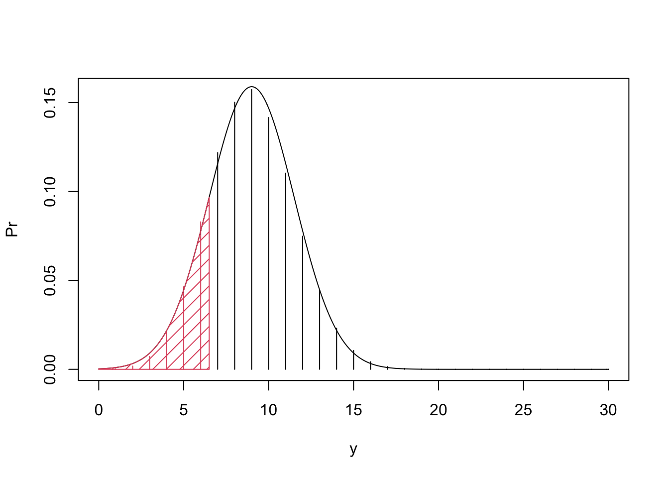
Figure 9.7: Normal Approximation of the Binomial Distribution

In principle, the Normal approximation is valid when \(n\), the number of independent trials in the Binomial distribution, is large. When \(n\) is relatively small the approximation may not be so good. Indeed, take \(Y \sim \mathrm{Binomial}(30,0.3)\) and consider the probability \(\operatorname{P}(Y \leq 6)\). Compare the actual probability to the Normal approximation:

pbinom(6,30,0.3)
#> [1] 0.159523
pnorm(6,30*0.3,sqrt(30*0.3*0.7))
#> [1] 0.1159989

The Normal approximation, which is equal to 0.1159989, is not too close to the actual probability, which is equal to 0.1595230.

A naïve application of the Normal approximation for the \(\mathrm{Binomial}(n,p)\) distribution may not be so good when the number of trials \(n\) is small. Yet, a small modification of the approximation may produce much better results. In order to explain the modification consult Figure 9.7 where you will find the bar plot of the Binomial distribution with the density of the approximating Normal distribution superimposed on top of it. The target probability is the sum of heights of the bars that are painted in red. In the naïve application of the Normal approximation we used the area under the normal density which is to the left of the bar associated with the value \(y=6\).

Alternatively, you may associate with each bar located at \(y\) the area under the normal density over the interval \([y-0.5, y+0.5]\). The resulting correction to the approximation will use the Normal probability of the event \(\{Y \leq 6.5\}\), which is the area shaded in red. The application of this approximation, which is called continuity correction produces:

pnorm(6.5,30*0.3,sqrt(30*0.3*0.7))
#> [1] 0.1596193

Observe that the corrected approximation is much closer to the target probability, which is 0.1595230, and is substantially better that the uncorrected approximation which was 0.1159989. Generally, it is recommended to apply the continuity correction to the Normal approximation of a discrete distribution.

Consider the \(\mathrm{Binomial}(n,p)\) distribution. Another situation where the Normal approximation may fail is when \(p\), the probability of “Success” in the Binomial distribution, is too close to 0 (or too close to 1). Recall, that for large \(n\) the Poisson distribution emerged as an approximation of the Binomial distribution in such a setting. One may expect that when \(n\) is large and \(p\) is small then the Poisson distribution may produce a better approximation of a Binomial probability. When the Poisson distribution is used for the approximation we call it a Poisson Approximation.

Let us consider an example. Let us analyze 3 Binomial distributions. The expectation in all the distributions is equal to 2 but the number of trials, \(n\), vary. In the first case \(n=20\) (and hence \(p=0.1\)), in the second \(n=200\) (and \(p=0.01\)), and in the third \(n=2,000\) (and \(p=0.001\). In all three cases we will be interested in the probability of obtaining a value less or equal to 3.

The Poisson approximation replaces computations conducted under the Binomial distribution with Poisson computations, with a Poisson distribution that has the same expectation as the Binomial. Since in all three cases the expectation is equal to 2 we get that the same Poisson approximation is used to the three probabilities:

ppois(3,2)
#> [1] 0.8571235

The actual Binomial probability in the first case (\(n=20\), \(p=0.1\)) and a Normal approximation thereof are:

pbinom(3,20,0.1)
#> [1] 0.8670467
pnorm(3.5,2,sqrt(20*0.1*0.9))
#> [1] 0.8682238

Observe that the Normal approximation (with a continuity correction) is better than the Poisson approximation in this case.

In the second case (\(n=200\), \(p=0.01\)) the actual Binomial probability and the Normal approximation of the probability are:

pbinom(3,200,0.01)
#> [1] 0.858034
pnorm(3.5,2,sqrt(200*0.01*0.99))
#> [1] 0.856789

Observe that the Poisson approximation that produces 0.8571235 is slightly closer to the target than the Normal approximation. The greater accuracy of the Poisson approximation for the case where \(n\) is large and \(p\) is small is more pronounced in the final case (\(n=2000\), \(p=0.001\)) where the target probability and the Normal approximation are:

pbinom(3,2000,0.001)
#> [1] 0.8572138
pnorm(3.5,2,sqrt(2000*0.001*0.999))
#> [1] 0.8556984

Compare the actual Binomial probability, which is equal to 0.8572138, to the Poisson approximation that produced 0.8571235. The Normal approximation, 0.8556984, is slightly off, but is still acceptable.

9.4 Exercises

Consider the problem of establishing regulations concerning the maximum number of people who can occupy a lift. In particular, we would like to assess the probability of exceeding maximal weight when 8 people are allowed to use the lift simultaneously and compare that to the probability of allowing 9 people into the lift.

Assume that the total weight of 8 people chosen at random follows a normal distribution with a mean of 560kg and a standard deviation of 57kg. Assume that the total weight of 9 people chosen at random follows a normal distribution with a mean of 630kg and a standard deviation of 61kg.

1. What is the probability that the total weight of 8 people exceeds 650kg?⁵⁶

2. What is the probability that the total weight of 9 people exceeds 650kg?⁵⁷

3. What is the central region that contains 80% of distribution of the total weight of 8 people?⁵⁸

4. What is the central region that contains 80% of distribution of the total weight of 9 people?⁵⁹

---

Assume \(Y \sim \mbox{Binomial}(27,0.32)\). We are interested in the probability \(\operatorname{P}(Y > 11)\).

1. Compute the (exact) value of this probability.⁶⁰

2. Compute a Normal approximation to this probability, without a continuity correction.⁶¹

3. Compute a Normal approximation to this probability, with a continuity correction.⁶²

4. Compute a Poisson approximation to this probability.⁶³

9.5 Summary

Glossary

Normal Random Variable:

A bell-shaped distribution that is frequently used to model a measurement. The distribution is marked with \(\mathrm{Normal}(\mu,\sigma)\). Note that R uses \(\sigma\) also, and not \(\sigma^2\) for its p and q functions .

Standard Normal Distribution:

The \(\mathrm{Normal}(0,1)\). The distribution of standardized Normal measurement.

Percentile:

Given a percent \(p \cdot 100\%\) (or a probability \(p\)), the value \(y\) is the percentile of a random variable \(Y\) if it satisfies the equation \(\operatorname{P}(Y \leq y) = p\).

Normal Approximation of the Binomial:

Approximate computations associated with the Binomial distribution with parallel computations that use the Normal distribution with the same expectation and standard deviation as the Binomial.

Poisson Approximation of the Binomial:

Approximate computations associated with the Binomial distribution with parallel computations that use the Poisson distribution with the same expectation as the Binomial.