Creating an R Package
Creating an R Package
- 1 Introduction
- 2 Pre-workshop set-up
- 3 Git and GitHub
- 4 Building an
Rpackage- 4.1 Package Structure
- 4.2 Getting Started
- 4.2.1 Step 1: Check working directory
- 4.2.2 Step 2: Add required
Rpackage files - 4.2.3 Step 3: Configure
RStudiobuild options - 4.2.4 Step 4: Build and install
- 4.2.5 Step 5: Fill in the blanks and commit changes
- 4.2.6 Step 6: Add a dataset
- 4.2.7 Step 7: Document the dataset
- 4.2.8 Step 8: Add an
Rfunction - 4.2.9 Step 9: Document the
Rfunction - 4.2.10 Step 10: Dependencies: What does your package need?
- 4.2.11 Step 11: Check your package
- 5 Vignettes
- 6 Continous Integration
- 7 Tests
- 8 Documentation
- 9
devtoolsfunctions - 10
usethisfunctions - 11 Resources
- References
1 Introduction
One of the fundamental roles of a statistician is to create methods to analyze data. This typically involves four components: developing the theory, translating the equations to computer code, a simulation study and a real data analysis. While these are enough to get published, it is unlikely your method will be used by others without a key fifth component: a software package. A package is a collection of reusable functions, the documentation that describes how to use them, tests and sample data. They provide a structured way to organize, use and distribute code to others and/or your future self. The objective of this workshop is to learn how to develop an R package. In addition to creating an R package from scratch, you will learn how to make it robust across platforms and future changes using continuous integration and unit testing. This workshop assumes familiarity with R, RStudio, writing functions, installing packages, loading libraries and requires a GitHub account. This will be an interactive workshop.
2 Pre-workshop set-up
You must bring your own laptop. It is vital that you attempt to set up your system in advance. You cannot show up at the workshop with no preparation and keep up!
- R (version ≥ 3.6.0)
- RStudio (version ≥ 1.2.1335). This is a powerful graphical user interface (GUI) which makes the package creation process much easier.
- Git. I strongly recommend reading these setup instructions by Jenny Bryan for Mac/Windows/Linux and the Troubleshooting section.
- Please read Chapter 1: Why Git? Why GitHub? to understand the big picture and motivation for using Git and Github.
- Sign up for a GitHub account. We will use GitHub to host the source files of our
Rpackage. I also recommend reading Jenny Bryan’s advice on carefully choosing a username.
- GitKraken. This is a GUI for Git which makes it much easier to dive into version control without the command line. GitKraken is to Git what RStudio is to R. This is optional but highly recommended, particularly for new Git users. You are free to use the GUI of your choice or simply the command line. In this workshop I will be using GitKraken.
- Complete Section 3 of this tutorial.
- Run the following commands in
R:
install.packages("pacman")
# this command checks if you have the packages already installed,
# then installs the missing packages, then loads the libraries
pacman::p_load(knitr, rmarkdown, devtools, roxygen2, usethis)
# identify yourself to Git with the usethis package
# use the exact same username and email associated
# with your GitHub account
usethis::use_git_config(user.name = "gauss", user.email = "gauss@normal.org")3 Git and GitHub
3.1 Introduction
This section walks you through the process of creating a GitHub repository (abbreviated as repo), creating a local copy of the repo (i.e. on your laptop), making some changes locally and updating your changes on the remote (aka GitHub repo). It assumes that you have successfully completed the requirements outlined in Section 2. The following figure summarizes some key terminology that we will make use of in this section:

Figure 3.1: source: http://ohi-science.org/data-science-training/
3.2 Annotations
For each step, I have provided screenshots annotated with red rectangles, circles and arrows. You can click on each image to enlarge it. The following table describes what each of the annotations represent.
| Annotation | Description |
|---|---|
 |
Enter text or fill in the blank |
 |
Click on the circled button |
| Take note of. No action is required. |
3.3 Step 1: Create a remote repo
We first create a GitHub repo. Head over to https://github.com and login. Then click on new repository:

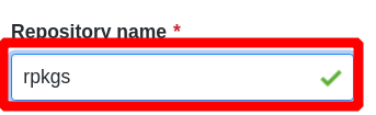
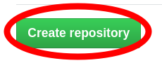
Give it a name. It can be anything you want (just pick a name that will remind you that this repository contains the source files of your R package). In the screenshots below I used rpkg throughout. Click on Create repository:

Copy the link of your newly created repo to your clipboard:

3.4 Step 2: New RStudio Project via git clone
Create a local copy of the remote repo using RStudio projects:

Click on Version Control:

Click on Git. Note that if you get an error or you don’t see this option, this likely means that your RStudio doesn’t know where to find your local Git installation. Please see Chapter 13: Detect Git from RStudio for troubleshooting this.

Paste the link to your remote repo in the Repository URL box, name the folder that will contain your R package files, and browse to where you want the folder to be saved in your filesystem. Click on Create Project:

Your RStudio window should open a new project in the specfied directory. Take note of the following points annotated in the screenshot below:
- The
Gittab allows you to useGitand push toGitHubwithinRStudio. You will see any changes that have been made to your files since the last commit here. I have found theRStudiointerface toGitto be inadequate and slow. I just want you to be aware of this functionality. I only look at this tab to quickly see if there were any changes, but do all my version controlling and interfacing withGitHubusingGitKraken. - Shows the path of your working directory, which is set to the root of your
RStudioproject by default. You can always click on the arrow to return to the working directory. - Indicates the name of your
Rstudioproject. It’s also a dropdown menu for other recently openedRStudioprojects. - Filesystem viewer of your working directory. You should see a
.gitignorefile and theRStudioproject file. These were automatically added byRStudiowhen you created a new project from aGitHubrepo. - A dropdown menu with extended
Gitfunctionalities.

3.5 Step 3: add and commit your changes
The following figure shows the commands needed for a basic version controlled workflow. Refer back to this figure once you complete Step 3 and then once again when you complete Step 4 (it should make a little more sense).

Figure 3.2: source: https://www.edureka.co/blog/git-tutorial/
Have you ever versioned a file by adding your initials or the date? That is effectively a commit, albeit only for a single file: it is a version that is significant to you and that you might want to inspect or revert to later (Bryan, STAT545TAs, and Hester 2019). The commit command is used to save your changes to the local repository. From the Git tab, click on Commit:

Note that you have to explicitly tell Git which changes you want to include in a commit before running the git commit command. This means that a file won’t be automatically included in the next commit just because it was changed. Instead, you need to use the git add command to mark the desired changes for inclusion. Instead of typing git add in the terminal, you can simply click the boxes next to the files you want to add (this is also referred to as staging a file). The lines 1 to 4 highlighted in green refer to the contents of the .gitignore file and the green highlight indicates they are being added to the file (red highlight indicates removal of a line):

Every time you make a commit you must also write a short commit message. Ideally, this conveys the motivation for the change. Remember, the diff will show the content. When you revisit a project after a break or need to digest recent changes made by a colleague, looking at the history, by reading commit messages and skimming through diffs, is an extremely efficient way to get up to speed (Bryan, STAT545TAs, and Hester 2019). Enter a commit message and click on the Commit button:

If everything worked, you should see the following screen with the commit message and the files that were added:

3.6 Step 4: push your local commits
The push command is used to publish new local commits on a remote server (the remote repo you created in Step 1):

Enter your username:

and your password:

Note the following:
- The URL of the remote repo.
- The name of the local branch called
master. (We’ll talk about branches later). - The name of the remote branch also called
master.master -> masterindicates that you have pushed the commit from the localmasterbranch to the remotemasterbranch. - The command you can enter in the terminal instead of using the
RStudiointerface topushyour commit to theremote.

Head over to your remote GitHub repo and take note of the following:
- The newly added files.
- The
commitmessage. - You are currently viewing the contents of the
masterbranch. - The unique ID of the
commit. A Git commit ID is a SHA-1 hash of every important thing about the commit. Clicking on it will allow you to see the difference (akadiff) between the previous commit. - The number of commits (aka snapshots of the repo).
- The number of branches.

3.7 Step 5: Open the repo with GitKraken
Link your GitHub account to GitKraken; you will be prompted for this when opening the GitKraken application for the first time. Open the local repo created in Step 2:


The following screenshot shows the local repo in the GitKraken GUI. Note the following (which has similar attributes to the online GitHub repo):
- The newly added files.
- The
commitmessage. - You are currently viewing the contents of the
masterbranch. - The unique ID of the
commit. A Git commit ID is a SHA-1 hash of every important thing about the commit. Clicking on it will allow you to see the difference (akadiff) between the previous commit. - The branches available locally.
- The branches available on the remote.

3.8 Discussion
Hopefully you were able to successfully complete all the steps in this Section. The main takeaway is to be able to add, commit, and push your local commits to the remote repo. It’s completely normal if you still have very little understanding of what just happened. I will clarify during the workshop. The point was for you to take a first stab at using version control and come to the workshop as prepared as possible.
4 Building an R package
This section runs through the development of a small toy package. It’s meant to illustrate the most important components of an R package. We will then provide a detailed treatment of the key components in the next sections.
4.1 Package Structure
A package is a convention for organizing files into directories. Figure 4.1 shows the 7 most common parts of
an R package.

Figure 4.1: source: https://rawgit.com/rstudio/cheatsheets/master/package-development.pdf
DESCRIPTIONfile (required): contains key metadata for the package that is used by repositories like CRAN and byRitself. This file contains the package name, the version number, the author and maintainer contact information, the license information, as well as any dependencies on other packages.NAMESPACEfile (required): specifies the interface to the package that is presented to the user. This is done via a series ofexport()statements, which indicate which functions in the package are exported to the user. Functions that are not exported cannot be called directly by the user (or they must use:::). In addition to exports, the NAMESPACE file also specifies what functions or packages are imported by the package. If your package depends on functions from another package, you must import them via the NAMESPACE file.Rsub-directory (required): The R sub-directory contains all of your R code, either in a single file, or in multiple files. For larger packages it’s usually best to split code up into multiple files that logically group functions together. The names of the R code files do not matter, but generally it’s not a good idea to have spaces in the file names.mansub-directory (required): contains the documentation files for all of the exported objects of a package. Theroxygen2package allows you to write the documentation directly into theRcode files. Therefore, you will likely have little interaction with themandirectory as all of the files in there will be auto-generated by theroxygen2package from theRcode files.testssub-directory: to store tests that will alert you if your code breaks.vignettessub-directory: holds documents that teach your users how to solve real problems with your tools.datasub-directory: allows you to include data with your package.
4.2 Getting Started
We will rely heavily on the following packages to build our own package:
usethis(Wickham and Bryan 2018) for setup and creating the required files and folders
devtools(Wickham, Hester, and Chang 2018) to build, install and check our package
roxygen2(Wickham, Danenberg, and Eugster 2018) to document our functions
rmarkdown(Xie, Allaire, and Grolemund 2018 ; Allaire et al. 2019) for creating package vignettes
4.2.1 Step 1: Check working directory
Ensure that your working directory is set to the root of the GitHub repo you created in Section 3. The following shows a plain text listing of the directory (at this stage, it should only contain two files):
-- .gitignore
-- rpkgs.Rproj4.2.2 Step 2: Add required R package files
Run the following commands in R from the root directory of your package:
# creates description and namespace files
usethis::use_description()
usethis::use_namespace()
# Create R directory
base::dir.create("R")
# creates Package-level documentation so you can run ?nameofpackage
usethis::use_package_doc()
# created README.Rmd for Github landing page
# an .Rbuildignore file gets created
usethis::use_readme_rmd()
# creates license file
usethis::use_mit_license("Sahir Bhatnagar")
# creates news file
usethis::use_news_md()
# setup continuous integration via travis-ci
usethis::use_travis()
# sets up testing infrastructure
usethis::use_testthat()Your package directory should now have the following structure:
-- .gitignore
-- .Rbuildignore
-- .travis.yml
-- DESCRIPTION
-- LICENSE
-- LICENSE.md
-- NAMESPACE
-- NEWS.md
-- R
|__rpkg-package.R
-- README.Rmd
-- rpkg.Rproj
-- tests
|__testthat
|__testthat.R4.2.3 Step 3: Configure RStudio build options
Restart RStudio. You should now see a Build tab:

Click on the .Rproj file:

Change the following options:


4.2.4 Step 4: Build and install
On the Build tab, click on Install and Restart or use Ctrl/Cmd + Shift + B:

This will install and load your package. Now enter the following commands:
?rpkg
rpkg::
pacman::p_functions(rpkg)You will notice that your package has a help page for the package by calling ?rpkg and also has no functions (given by pacman::p_functions()):

In the man folder you will see a rpkg-package.Rd file. This is an R documentation formatted file and is generated automatically by the roxygen2 package. We will talk more about documentation in the following sections.

4.2.5 Step 5: Fill in the blanks and commit changes
Exercise: Update the DESCRIPTION file and the README.Rmd file. Then rebuild the package. Add and commit your changes and push them to the remote repo. Check the commit history and the differences between the previous commit.
4.2.6 Step 6: Add a dataset
It’s often useful to include data in a package. If you’re releasing the package to a broad audience, it’s a way to provide compelling use cases for the package’s functions. Before I start writing functions for my packages, I usually add a toy dataset first. Enter the following R code:
# this will setup the folders needed for the data and raw-data
usethis::use_data_raw()The data-raw folder gets added to the .Rbuildignore so that it’s not shipped with the package. This folder is used to store the raw data and the scripts used to parse it and create the final version of the dataset.
For this exercise, we will use a data set on two-week seizure counts for 59 epileptics (or you can use your own). Download the raw .csv file and save it in the data-raw folder.
Create an R script called seizure-data.R and save it in the data-raw folder. This script will contain the code used to clean the dataset and ouput the final cleaned version to be shipped with the package. Enter the following code in the seizure-data.R script:
# load required packages ----
if (!require("pacman")) install.packages("pacman")
pacman::p_load(magrittr, dplyr, usethis, data.table, here)
# clean data ----
epil <- read.csv(here::here("data-raw","epil.csv"))
DT <- epil %>% as.data.table
DT.base <- DT %>% distinct(subject, .keep_all = TRUE)
DT.base[,`:=`(period=0,y=base)]
DT.epil <- rbind(DT, DT.base)
setkey(DT.epil, subject, period)
DT.epil[,`:=`(post=as.numeric(period>0), tj=ifelse(period==0,8,2))]
df_epil <- as.data.frame(DT.epil) %>% dplyr::select(y, trt, post, subject, tj)
# write data in correct format to data folder ----
usethis::use_data(df_epil, overwrite = TRUE)Exercise: Source the seizure-data.R script. Inspect the additions and then add and commit the changes.
4.2.7 Step 7: Document the dataset
Datasets must be documented. We usually document them in R/data.R. Enter the following in a file called data.R and save it in the R folder:
#' Seizure Counts for Epileptics
#'
#' @description Thall and Vail (1990) give a data set on two-week
#' seizure counts for 59 epileptics. The number of seizures was
#' recorded for a baseline period of 8 weeks, and then patients
#' were randomly assigned to a treatment group or a control group.
#' Counts were then recorded for four successive two-week periods.
#' The subject's age is the only covariate.
#'
#' @format his data frame has 295 rows and the following 5 columns:
#' \describe{
#' \item{y}{the count for the 2-week period.}
#' \item{trt}{treatment, "placebo" or "progabide"}
#' \item{post}{post treatment. 0 for no, 1 for yes}
#' \item{subject}{subject id}
#' \item{tj}{time}
#' }
#' @source \url{https://cran.r-project.org/package=MASS}
"df_epil"You can also document multiple datasets in the same R file (see here for an example). Refer to the Documentation section for more details on roxygen2 tags.
Exercise: Re-build the package. Check out the help page for the df_epil dataset using ?df_epil. Inspect the additions and then add and commit the changes.
4.2.8 Step 8: Add an R function
To make our package actually useful, we need to add an R function. I use the following function for the purposes of illustration, which analyzes the data and outputs a summary of the results in the form of an HTML table. Save this function in R/fit_models:
fit_models <- function(formula, data) {
fit.glmm <- lme4::glmer(formula,
data = data,
family = "poisson",
offset = log(tj))
sjPlot::tab_model(fit.glmm)
}
# example of how to use the function
# fit_models(formula = y ~ trt*post + (1|subject), data = df_epil)4.2.9 Step 9: Document the R function
We again make use of the roxygen2 package to document our R function. The sinew (Sidi 2018) package creates a skeleton for us. Enter the following commands in R to document the function:
pacman::p_load(sinew)
sinew::makeOxyFile("R/fit_models.R")Exercise: Delete the R/fit_models.R file and rename R/oxy-fit_models.R to R/fit_models.R. Fill in the roxygen2 template (refer to the Section on documentation for more details). Re-build the package. Check out the help page for the fit_models function using ?fit_models. Inspect the additions and then add and commit the changes. Push to the remote repo.
4.2.10 Step 10: Dependencies: What does your package need?
See complete references on DESCRIPTION and NAMESPACE.
It’s the job of the DESCRIPTION to list the packages that your package needs to work. R has a rich set of ways of describing potential dependencies. For example, the following lines indicate that my package needs both lme4 and sjPlot to work:
Imports:
lme4,
sjPlotWhereas, the lines below indicate that while my package can take advantage of lme4 and sjPlot, they’re not required to make it work:
Suggests:
lme4,
sjPlotBoth Imports and Suggests take a comma separated list of package names. I recommend putting one package on each line, and keeping them in alphabetical order. That makes it easy to skim.
Imports and Suggests differ in their strength of dependency:
Imports: packages listed here must be present for your package to work. In fact, any time your package is installed, those packages will, if not already present, be installed on your computer (devtools::load_all()also checks that the packages are installed).
Adding a package dependency in Imports ensures that it’ll be installed. However, it does not mean that it will be attached along with your package (i.e., library(x)). The best practice is to explicitly refer to external functions using the syntax package::function(). This makes it very easy to identify which functions live outside of your package. This is especially useful when you read your code in the future.
Suggests: your package can use these packages, but doesn’t require them. You might use suggested packages for example datasets, to run tests, build vignettes, or maybe there’s only one function that needs the package. Packages listed in Suggests are not automatically installed along with your package. This means that you need to check if the package is available before using it (use requireNamespace(x, quietly = TRUE)). There are two basic scenarios:
# You need the suggested package for this function
my_fun <- function(a, b) {
if (!requireNamespace("pkg", quietly = TRUE)) {
stop("Package \"pkg\" needed for this function to work. Please install it.",
call. = FALSE)
}
}
# There's a fallback method if the package isn't available
my_fun <- function(a, b) {
if (requireNamespace("pkg", quietly = TRUE)) {
pkg::f()
} else {
g()
}
}The easiest way to add Imports and Suggests to your package is to use:
usethis::use_package("lme4", type = "Imports")
usethis::use_package("lme4", type = "Suggests")This automatically puts them in the right place in your DESCRIPTION, and reminds you how to use them.
It’s common for packages to be listed in Imports in DESCRIPTION, but not in NAMESPACE. In fact, this is what Hadley recommends: list the package in DESCRIPTION so that it’s installed, then always refer to it explicitly with pkg::fun(). The converse is not true. Every package mentioned in NAMESPACE must also be present in the Imports or Depends fields.
Exercise: Add lme4 and sjPlot to the DESCRIPTION. Re-build the package. Check out the help page for the package using ?rpkg. Inspect the additions and then add and commit the changes. Push to the remote repo.
4.2.11 Step 11: Check your package
R CMD check, executed in the terminal, is the gold standard for checking that an R package is in full working order. devtools::check() is a convenient way to run this without leaving your R session.
Exercise: Run devtools::check(). Fix the errors and rebuild the package. Add and commit your changes and push to remote repo.
5 Vignettes
You will likely want to create a document that walks users through the basics of how to use your package. You can do this through two formats:
- Vignette: This document is bundled with your
Rpackage, so it becomes locally available to a user once they install your package from CRAN. They will also have it available if they install the package from GitHub, as long as they use thebuild_vignettes = TRUEoption when runningremotes::install_github. - README file: If you have your package on GitHub, this document will show up on the main page of the repository if there is a
README.mdfile in the top directory of the repository. For an example, visit https://github.com/geanders/countytimezones and scroll down. You’ll see a list of all the files and subdirectories included in the package repository and below that is the content in the package’s README.md file, which gives a tutorial on using the package.
The README file is a useful way to give GitHub users information about your package, but it will not be included in builds of the package or be available through CRAN for packages that are posted there. Instead, if you want to create tutorials or overview documents that are included in a package build, you should do that by adding one or more package vignettes. Vignettes are stored in a vignettes subdirectory within the package directory.
To add a vignette file, saved within this subdirectory (which will be created if you do not already have it), use:
usethis::use_vignette(name = "Introduction to my package")Once you create a vignette with usethis::use_vignette, be sure to update the Vignette Index Entry in the vignette’s YAML (the code at the top of an R Markdown document). Replace Vignette Title there with the actual title you use for the vignette.
Exercise: Re-build the package. Inspect the additions and then add and commit the changes. Make sure the vignette is able to be compiled. Then push to the remote repo.
6 Continous Integration
The objectives of this section are:
- Create an R package that is tested and deployed on Travis
- Create an R package that is tested and deployed on Appveyor
Continous integration (aka checking your package after every commit) is a software development technique used to ensure that any changes to your code do not break the package’s functionality. Travis is a continuous integration service, which means that it runs automated testing code everytime you push to GitHub. For open source projects, Travis provides 50 minutes of free computation on a Ubuntu server for every push. For an R package, the most useful code to run is devtools::check().
When it comes to R packages continuous integration means ensuring that your package builds without any errors or warnings, and making sure that all of the tests that you’ve written for your package are passing. Building your R package will protect you against some big errors, but the best way that you can ensure continuous integration will be useful to you is if you build robust and complete tests for every function in your package.
6.1 Travis and Appveyor
Travis will test your package on Linux, and AppVeyor will test your package on Windows. Both of these services are free for R packages that are built in public GitHub repositories. These continuous integration services will run every time you push a new set of commits for your package repository. Both services integrate nicely with GitHub so you can see in GitHub’s pull request pages whether or not your package is building correctly.
6.1.1 Using Travis
To start using Travis:
- Go to https://travis-ci.org and sign in with your GitHub account.
- Ensure that you have run
usethis::use_travis(). - Clicking on your name in the upper right hand corner of the site will bring up a list of your public GitHub repositories with a switch next to each repo. If you turn the switch on then the next time you push to that repository Travis will look for a
.travis.ymlfile in the root of the repository, and it will run tests on your package accordingly. - Now add, commit, and push your changes to GitHub, which will trigger the first build of your package on Travis. Go back to https://travis-ci.org to watch your package be built and tested at the same time! You may want to make some changes to your .travis.yml file, and you can see all of the options available in this guide.
Once your package has been built for the first time you’ll be able to obtain a badge, which is just a small image generated by Travis which indicates whether you package is building properly and passing all of your tests. You should display this badge in the README.Rmd file of your package’s GitHub repository so that you and others can monitor the build status of your package (you should see the code for the badge appear in your console once you use usethis::use_travis()).
6.1.2 Using AppVeyor
To start using AppVeyor:
- Go to https://www.appveyor.com/ and sign in with your GitHub account.
- Ensure that you have run
usethis::use_appveyor(). This command will set up a defaultappveyor.ymlfor yourRpackage - After signing in click on
Projectsin the top navigation bar. If you have any GitHub repositories that use AppVeyor you’ll be able to see them here. To add a new project clickNew Projectand find the GitHub repo that corresponds to theRpackage you’d like to test on Windows. ClickAddfor AppVeyor to start tracking this repo. - Now add, commit, and push your changes to GitHub, which will trigger the first build of your package on AppVeyor.
- Go back to https://www.appveyor.com/ to see the result of the build. You may want to make some changes to your appveyor.yml file, and you can see all of the options available in the r-appveyor guide which is maintained by Kirill Müller.
- Like Travis, AppVeyor also generates badges that you should add to the README.Rmd file of your package’s GitHub repository (you should see the code for the badge appear in your console once you use
usethis::use_appveyor())
Exercise: Re-build the package. Inspect the additions and then add and commit the changes. Then push to the remote repo.
7 Tests
See complete reference.
What to test: Whenever you are tempted to type something into a print statement or a debugger expression, write it as a test instead. — Martin Fowler
Testing is a vital part of package development. It ensures that your code does what you want it to do. Testing, however, adds an additional step to your development workflow. The goal of this section is to show you how to make this task easier and more effective by doing formal automated testing using the testthat package.
The testthat package is designed to make it easy to setup a battery of tests for your R package. A nice introduction to the package can be found in Hadley Wickham’s article in the R Journal. Essentially, the package contains a suite of functions for testing function/expression output with the expected output. Add the following to tests/testthat/test-fit_models.R:
context("run fit_model with packaged dataset df_epil")
data("df_epil")
fit <- try(fit_models(formula = y ~ trt*post + (1|subject), data = df_epil),
silent = TRUE)
test_that("no error in fitting fit_models for the epilepsy data", {
expect_false(inherits(fit, "try-error"))
})Then run the following commands in R:
# execute the test
devtools::test()
# use code coverage
usethis::use_coverage()
# check code coverage
devtools::test_coverage()Exercise: Re-build the package. Run devtools::check(). Fix any errors. Inspect the additions and then add and commit the changes. Then push to the remote repo.
7.1 Another example
Exercise: Document the following function and write a test for it. Think about checking for a positive definite covariance matrix and create a function for this check.
sim.expr.data <- function(n, n0, p, rho.0, rho.1){
# Initiate Simulation parameters
# n: total number of subjects
# n0: number of subjects with X=0
# n1: number of subjects with X=1
# p: number of genes
# rho.0: rho between Z_i and Z_j when X=0
# rho.1: rho between Z_i and Z_j when X=1
# Simulate gene expression values according to exposure X=0, X=1,
# according to a centered multivariate normal distribution with
# covariance between Z_i and Z_j being rho^|i-j|
times = 1:p # used for creating covariance matrix
H <- abs(outer(times, times, "-"))
V0 <- rho.0^H
V1 <- rho.1^H
# rows are people, columns are genes
genes0 <- MASS::mvrnorm(n = n0, mu = rep(0,p), Sigma = V0)
genes1 <- MASS::mvrnorm(n = n1, mu = rep(0,p), Sigma = V1)
genes <- rbind(genes0,genes1)
colnames(genes) <- paste0("Gene", 1:p)
rownames(genes) <- paste0("Subject", 1:n)
return(genes)
}
genes <- sim.expr.data(n = 100, n0 = 50, p = 100,
rho.0 = 0.01, rho.1 = 0.95)
# checking for positive definite matrix called tt
if (!all(eigen(tt)$values > 0)) {
message("eta * sigma2 * kin not PD, using Matrix::nearPD")
tt <- Matrix::nearPD(tt)$mat
}8 Documentation
In RStudio, go to Help --> Roxygen Quick Reference
Refer to Table 8.1 and Table 8.2 for a summary of the most commonly used roxygen2 tags and formatting tags for creating function documentation.
| Tag | Meaning |
|---|---|
| @return | A description of the object returned by the function |
| @parameter | Explanation of a function parameter |
| @inheritParams | Name of a function from which to get parameter definitions |
| @examples | Example code showing how to use the function |
| @details | Add more details on how the function works (for example, specifics of the algorithm being used) |
| @note | Add notes on the function or its use |
| @source | Add any details on the source of the code or ideas for the function |
| @references | Add any references relevant to the function |
| @importFrom | Import a function from another package to use in this function (this is especially useful for inline functions like %>% and %within%) |
| @export | Export the function, so users will have direct access to it when they load the package |
| Tag | Meaning |
|---|---|
| \code{} | Format in a typeface to look like code |
| \dontrun{} | Use with examples, to avoid running the example code during package builds and testing |
| \link{} | Link to another R function |
| \eqn{}{} | Include an inline equation |
| \deqn{}{} | Include a display equation (i.e., shown on its own line) |
| \itemize{} | Create an itemized list |
| \url{} | Include a web link |
| \href{}{} | Include a web link |
9 devtools functions
Here are some of the key functions included in devtools and what they do, roughly in the order you are likely to use them as you develop an R package:
| Function | Use |
|---|---|
| load_all | Load the code for all functions in the package |
| document | Create documentation files and the “NAMESPACE” file from roxygen2 code |
| check | Check the full R package for any ERRORs, WARNINGs, or NOTEs |
| build_win | Build a version of the package for Windows and send it to be checked on a Windows machine. You’ll receive an email with a link to the results. |
| submit_cran | Submit the package to CRAN |
10 usethis functions
Here are some of the key functions included in usethis and what they do:
| Function | Use |
|---|---|
| use_data | Save an object in your R session as a dataset in the package |
| use_description | Set up the package to include a DESCRIPTION file |
| use_namespace | Set up the package to include a NAMESPACE file |
| use_vignette | Set up the package to include a vignette |
| use_travis | Set up travis ci |
| use_appveyor | Set up appveyor |
| use_testthat | Set up folders for testing |
| use_test | Create test file named by the function argument in the correct folder |
| use_readme_rmd | Set up the package to include a README file in Rmarkdown format |
| use_build_ignore | Specify files that should be ignored when building the R package (for example, if you have a folder where you’re drafting a journal article about the package, you can include all related files in a folder that you set to be ignored during the package build) |
| use_cran_comments | Create a file where you can add comments to include with your CRAN submission. |
| use_news_md | Add a file to the package to give news on changes in new versions |
11 Resources
References
Allaire, JJ, Yihui Xie, Jonathan McPherson, Javier Luraschi, Kevin Ushey, Aron Atkins, Hadley Wickham, Joe Cheng, Winston Chang, and Richard Iannone. 2019. Rmarkdown: Dynamic Documents for R. https://rmarkdown.rstudio.com.
Bryan, Jenny, STAT545TAs, and Jim Hester. 2019. Happy Git and Github for the useR. https://happygitwithr.com/.
Peng, Roger, Sean Kross, and Brooke Anderson. 2017. Mastering Software Development in R. https://bookdown.org/rdpeng/RProgDA/.
Sidi, Jonathan. 2018. Sinew: Create ’Roxygen2’ Skeleton with Information from Function Script. https://CRAN.R-project.org/package=sinew.
Wickham, Hadley, and Jennifer Bryan. 2018. Usethis: Automate Package and Project Setup. https://CRAN.R-project.org/package=usethis.
Wickham, Hadley, Peter Danenberg, and Manuel Eugster. 2018. Roxygen2: In-Line Documentation for R. https://CRAN.R-project.org/package=roxygen2.
Wickham, Hadley, Jim Hester, and Winston Chang. 2018. Devtools: Tools to Make Developing R Packages Easier. https://CRAN.R-project.org/package=devtools.
Xie, Yihui, J.J. Allaire, and Garrett Grolemund. 2018. R Markdown: The Definitive Guide. Boca Raton, Florida: Chapman; Hall/CRC. https://bookdown.org/yihui/rmarkdown.