Plot Hazards and Hazard Ratios
Source:R/plotHazardRatio.R, R/plot_methods.R, R/utils.R
plot.singleEventCB.RdPlot method for objects returned by the fitSmoothHazard
function. Current plot types are hazard function and hazard ratio. The
visreg package must be installed for type="hazard". This
function accounts for the possible time-varying exposure effects.
plotHazardRatio(x, newdata, newdata2, ci, ci.lvl, ci.col, rug, xvar, ...)

# S3 method for class 'singleEventCB'
plot(
  x,
  ...,
  type = c("hazard", "hr"),
  hazard.params = list(),
  newdata,
  exposed,
  increment = 1,
  var,
  xvar = NULL,
  ci = FALSE,
  ci.lvl = 0.95,
  rug = !ci,
  ci.col = "grey"
)

incrVar(var, increment = 1)
Arguments
- x
Fitted object of class
glm,gam,cv.glmnetorgbm. This is the result from thefitSmoothHazard()function.- newdata
Required for
type="hr". Thenewdataargument is the "unexposed" group, while the exposed group is defined by either: (i) a change (defined by theincrementargument) in a variable in newdata defined by thevarargument ; or (ii) an exposed function that takes a data-frame and returns the "exposed" group (e.g.exposed = function(data) transform(data, treat=1)). This is a generalization of the behavior of the rstpm2 plot function. It allows both numeric and factor variables to be incremented or decremented. See references for rstpm2 package. Only used fortype="hr"- newdata2
data.framefor exposed group. calculated and passed internally toplotHazardRatiofunction- ci
Logical; if TRUE confidence bands are calculated. Only available for
family="glm"andfamily="gam", and only used fortype="hr", Default: !add. Confidence intervals for hazard ratios are calculated using the Delta Method.- ci.lvl
Confidence level. Must be in (0,1), Default: 0.95. Only used for
type="hr".- ci.col
Confidence band color. Only used if argument
ci=TRUE, Default: 'grey'. Only used fortype="hr".- rug
Logical. Adds a rug representation (1-d plot) of the event times (only for
status=1), Default: !ci. Only used fortype="hr".- xvar
Variable to be used on x-axis for hazard ratio plots. If NULL, the function defaults to using the time variable used in the call to
fitSmoothHazard. In general, this should be any continuous variable which has an interaction term with another variable. Only used fortype="hr".- ...
further arguments passed to
plot. Only used iftype="hr". Any oflwd,lty,col,pch,cexwill be applied to the hazard ratio line, or point (if only one time point is supplied tonewdata).- type
plot type. Choose one of either
"hazard"for hazard function or"hr"for hazard ratio. Default:type = "hazard".- hazard.params
Named list of arguments which will override the defaults passed to
visreg::visreg(), The default arguments arelist(fit = x, trans = exp, plot = TRUE, rug = FALSE, alpha = 1, partial = FALSE, overlay = TRUE). For example, if you want a 95% confidence band, specifyhazard.params = list(alpha = 0.05). Note that Thecondargument must be provided as a named list. Each element of that list specifies the value for one of the terms in the model; any elements left unspecified are filled in with the median/most common category. Only used fortype="hazard". All other argument are used fortype="hr". Note that thevisregpackage must be installed fortype="hazard".- exposed
function that takes
newdataand returns the exposed dataset (e.g. function(data) transform(data, treat = 1)). This argument takes precedence over thevarargument, i.e., if bothvarandexposedare correctly specified, only theexposedargument will be used. Only used fortype="hr".- increment
Numeric value indicating how much to increment (if positive) or decrement (if negative) the
varvariable innewdata. Seevarargument for more details. Default is 1. Only used fortype="hr".- var
specify the variable name for the exposed/unexposed (name is given as a character variable). If this argument is missing, then the
exposedargument must be specified. This is the variable which will be incremented by theincrementargument to give the exposed category. Ifvaris coded as a factor variable, thenincrement=1will return the next level of the variable innewdata.increment=2will return two levels above, and so on. If the value supplied toincrementis greater than the number of levels, this will simply return the max level. You can also decrement the categorical variable by specifying a negative value, e.g.,increment=-1will return one level lower than the value innewdata. Ifvaris a numeric, thanincrementwill increment (if positive) or decrement (if negative) by the supplied value. Only used fortype="hr".
Value
a plot of the hazard function or hazard ratio. For type="hazard", a
data.frame (returned invisibly) of the original data used in the fitting
along with the data used to create the plots including predictedhazard
which is the predicted hazard for a given covariate pattern and time.
predictedloghazard is the predicted hazard on the log scale. lowerbound
and upperbound are the lower and upper confidence interval bounds on the
hazard scale (i.e. used to plot the confidence bands). standarderror is
the standard error of the log hazard or log hazard ratio (only if
family="glm" or family="gam"). For type="hr", log_hazard_ratio and
hazard_ratio is returned, and if ci=TRUE, standarderror (on the log
scale) and lowerbound and upperbound of the hazard_ratio are
returned.
Details
This function has only been thoroughly tested for family="glm". If
the user wants more customized plot aesthetics, we recommend saving the
results to a data.frame and using the graphical package of their choice.
References
Mark Clements and Xing-Rong Liu (2019). rstpm2: Smooth Survival Models, Including Generalized Survival Models. R package version 1.5.1. https://CRAN.R-project.org/package=rstpm2
Breheny P and Burchett W (2017). Visualization of Regression Models Using visreg. The R Journal, 9: 56-71.
See also
Examples
if (requireNamespace("splines", quietly = TRUE)) {
data("simdat") # from casebase package
library(splines)
simdat <- transform(simdat[sample(1:nrow(simdat), size = 200),],
treat = factor(trt, levels = 0:1,
labels = c("control","treatment")))
fit_numeric_exposure <- fitSmoothHazard(status ~ trt*bs(eventtime),
data = simdat,
ratio = 1,
time = "eventtime")
fit_factor_exposure <- fitSmoothHazard(status ~ treat*bs(eventtime),
data = simdat,
ratio = 1,
time = "eventtime")
newtime <- quantile(fit_factor_exposure[["data"]][[fit_factor_exposure[["timeVar"]]]],
probs = seq(0.05, 0.95, 0.01))
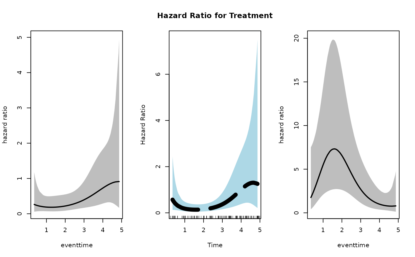
par(mfrow = c(1,3))
plot(fit_numeric_exposure,
type = "hr",
newdata = data.frame(trt = 0, eventtime = newtime),
exposed = function(data) transform(data, trt = 1),
xvar = "eventtime",
ci = TRUE)
#by default this will increment `var` by 1 for exposed category
plot(fit_factor_exposure,
type = "hr",
newdata = data.frame(treat = factor("control",
levels = c("control","treatment")), eventtime = newtime),
var = "treat",
increment = 1,
xvar = "eventtime",
ci = TRUE,
ci.col = "lightblue",
xlab = "Time",
main = "Hazard Ratio for Treatment",
ylab = "Hazard Ratio",
lty = 5,
lwd = 7,
rug = TRUE)
# we can also decrement `var` by 1 to give hazard ratio for control/treatment
result <- plot(fit_factor_exposure,
type = "hr",
newdata = data.frame(treat = factor("treatment",
levels = c("control","treatment")),
eventtime = newtime),
var = "treat",
increment = -1,
xvar = "eventtime",
ci = TRUE)
# see data used to create plot
head(result)
}
 #> treat eventtime log_hazard_ratio standarderror hazard_ratio lowerbound
#> 5% treatment 0.3488444 0.5617254 0.7422200 1.753696 0.4094260
#> 6% treatment 0.3902785 0.6649501 0.7012281 1.944394 0.4919237
#> 7% treatment 0.4148271 0.7239973 0.6788513 2.062662 0.5452413
#> 8% treatment 0.4512202 0.8086798 0.6482910 2.244942 0.6300556
#> 9% treatment 0.4636149 0.8367497 0.6385929 2.308850 0.6604266
#> 10% treatment 0.4862850 0.8870854 0.6217826 2.428043 0.7177844
#> upperbound
#> 5% 7.511610
#> 6% 7.685473
#> 7% 7.803102
#> 8% 7.998922
#> 9% 8.071737
#> 10% 8.213317
#> treat eventtime log_hazard_ratio standarderror hazard_ratio lowerbound
#> 5% treatment 0.3488444 0.5617254 0.7422200 1.753696 0.4094260
#> 6% treatment 0.3902785 0.6649501 0.7012281 1.944394 0.4919237
#> 7% treatment 0.4148271 0.7239973 0.6788513 2.062662 0.5452413
#> 8% treatment 0.4512202 0.8086798 0.6482910 2.244942 0.6300556
#> 9% treatment 0.4636149 0.8367497 0.6385929 2.308850 0.6604266
#> 10% treatment 0.4862850 0.8870854 0.6217826 2.428043 0.7177844
#> upperbound
#> 5% 7.511610
#> 6% 7.685473
#> 7% 7.803102
#> 8% 7.998922
#> 9% 8.071737
#> 10% 8.213317