Fit Linear Mixed Model with Lasso or Group Lasso Regularization

Main function to fit the linear mixed model with lasso or group lasso penalty for a sequence of tuning parameters. This is a penalized regression method that accounts for population structure using either the kinship matrix or the factored realized relationship matrix

ggmix(
  x,
  y,
  U,
  D,
  kinship,
  K,
  n_nonzero_eigenvalues,
  n_zero_eigenvalues,
  estimation = c("full"),
  penalty = c("lasso"),
  group,
  penalty.factor = rep(1, p_design),
  lambda = NULL,
  lambda_min_ratio = ifelse(n_design < p_design, 0.01, 1e-04),
  nlambda = 100,
  eta_init = 0.5,
  maxit = 100,
  fdev = 1e-20,
  standardize = FALSE,
  alpha = 1,
  thresh_glmnet = 1e-08,
  epsilon = 1e-04,
  dfmax = p_design + 2,
  verbose = 0
)

Arguments

x	input matrix, of dimension n x p; where n is the number of observations and p are the number of predictors.
y	response variable. must be a quantitative variable
U	left singular vectors corresponding to the non-zero eigenvalues provided in the `D` argument.
D	non-zero eigenvalues. This option is provided to the user should they decide or need to calculate the eigen decomposition of the kinship matrix or the singular value decomposition of the matrix of SNPs used to calculate the kinship outside of this function. This may occur, if for example, it is easier (e.g. because of memory issues, it's easier to calculate in plink). This should correspond to the non-zero eigenvalues only. Note that if you are doing an `svd` on the matrix of SNPs used to calculate the kinship matrix, then you must provide the square of the singular values so that they correspond to the eigenvalues of the kinship matrix. If you want to use the low rank estimation algorithm, you must provide the truncated eigenvalues and eigenvectors to the `D` and `U` arguments, respectively. If you want `ggmix` to truncate the eigenvectors and eigenvalues for low rank estimation, then provide either `K` or `kinship` instead and specify `n_nonzero_eigenvalues`.
kinship	positive definite kinship matrix
K	the matrix of SNPs used to determine the kinship matrix
n_nonzero_eigenvalues	the number of nonzero eigenvalues. This argument is only used when `estimation="low"` and either `kinship` or `K` is provided. This argument will limit the function to finding the `n_nonzero_eigenvalues` largest eigenvalues. If `U` and `D` have been provided, then `n_nonzero_eigenvalues` defaults to the length of `D`.
n_zero_eigenvalues	Currently not being used. Represents the number of zero eigenvalues. This argument must be specified when `U` and `D` are specified and `estimation="low"`. This is required for low rank estimation because the number of zero eigenvalues and their corresponding eigenvalues appears in the likelihood. In general this would be the rank of the matrix used to calculate the eigen or singular value decomposition. When `kinship` is provided and `estimation="low"` the default value will be `nrow(kinship) - n_nonzero_eigenvalues`. When `K` is provided and `estimation="low"`, the default value is `rank(K) - n_nonzero_eigenvalues`
estimation	type of estimation. Currently only `type="full"` has been implemented.
penalty	type of regularization penalty. Currently, only penalty="lasso" has been implemented.
group	a vector of consecutive integers describing the grouping of the coefficients. Currently not implemented, but will be used when penalty="gglasso" is implemented.
penalty.factor	Separate penalty factors can be applied to each coefficient. This is a number that multiplies lambda to allow differential shrinkage. Can be 0 for some variables, which implies no shrinkage, and that variable is always included in the model. Default is 1 for all variables
lambda	A user supplied lambda sequence (this is the tuning parameter). Typical usage is to have the program compute its own lambda sequence based on nlambda and lambda.min.ratio. Supplying a value of lambda overrides this. WARNING: use with care. Do not supply a single value for lambda (for predictions after CV use predict() instead). Supply instead a decreasing sequence of lambda values. glmnet relies on its warms starts for speed, and its often faster to fit a whole path than compute a single fit.
lambda_min_ratio	Smallest value for lambda, as a fraction of lambda.max, the (data derived) entry value (i.e. the smallest value for which all coefficients are zero). The default depends on the sample size nobs relative to the number of variables nvars. If nobs > nvars, the default is 0.0001, close to zero. If nobs < nvars, the default is 0.01. A very small value of lambda.min.ratio will lead to a saturated fit in the nobs < nvars case.
nlambda	the number of lambda values - default is 100.
eta_init	initial value for the eta parameter, with $0 < \eta < 1$ used in determining lambda.max and starting value for fitting algorithm.
maxit	Maximum number of passes over the data for all lambda values; default is 10^2.
fdev	Fractional deviance change threshold. If change in deviance between adjacent lambdas is less than fdev, the solution path stops early. factory default = 1.0e-5
standardize	Logical flag for x variable standardization, prior to fitting the model sequence. The coefficients are always returned on the original scale. Default is standardize=FALSE. If variables are in the same units already, you might not wish to standardize.
alpha	The elasticnet mixing parameter, with $0 \leq \alpha \leq 1$. alpha=1 is the lasso penalty, and alpha=0 the ridge penalty.
thresh_glmnet	Convergence threshold for coordinate descent for updating beta parameters. Each inner coordinate-descent loop continues until the maximum change in the objective after any coefficient update is less than thresh times the null deviance. Defaults value is 1E-7
epsilon	Convergence threshold for block relaxation of the entire parameter vector $\Theta = ( \beta, \eta, \sigma^2 )$. The algorithm converges when $$crossprod(\Theta_{j+1} - \Theta_{j}) < \epsilon$$. Defaults value is 1E-4
dfmax	limit the maximum number of variables in the model. Useful for very large `p` (the total number of predictors in the design matrix), if a partial path is desired. Default is the number of columns in the design matrix + 2 (for the variance components)
verbose	display progress. Can be either 0,1 or 2. 0 will not display any progress, 2 will display very detailed progress and 1 is somewhere in between. Default: 0.

References

Bhatnagar, Sahir R, Yang, Yi, Lu, Tianyuan, Schurr, Erwin, Loredo-Osti, JC, Forest, Marie, Oualkacha, Karim, and Greenwood, Celia MT. (2020) Simultaneous SNP selection and adjustment for population structure in high dimensional prediction models https://doi.org/10.1101/408484

Friedman, J., Hastie, T. and Tibshirani, R. (2008) Regularization Paths for Generalized Linear Models via Coordinate Descent, http://www.stanford.edu/~hastie/Papers/glmnet.pdf Journal of Statistical Software, Vol. 33(1), 1-22 Feb 2010 http://www.jstatsoft.org/v33/i01/

Yang, Y., & Zou, H. (2015). A fast unified algorithm for solving group-lasso penalize learning problems. Statistics and Computing, 25(6), 1129-1141. http://www.math.mcgill.ca/yyang/resources/papers/gglasso.pdf

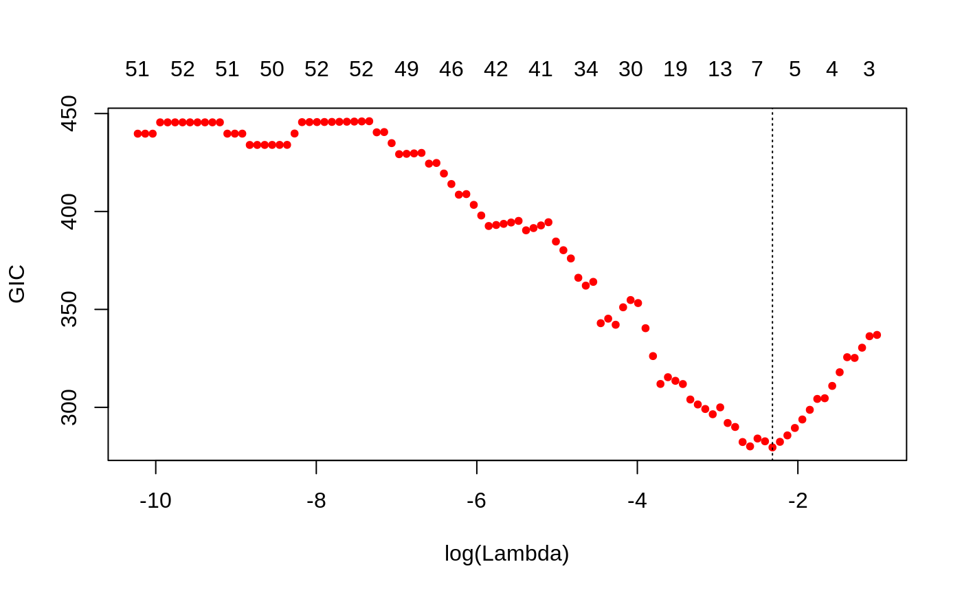
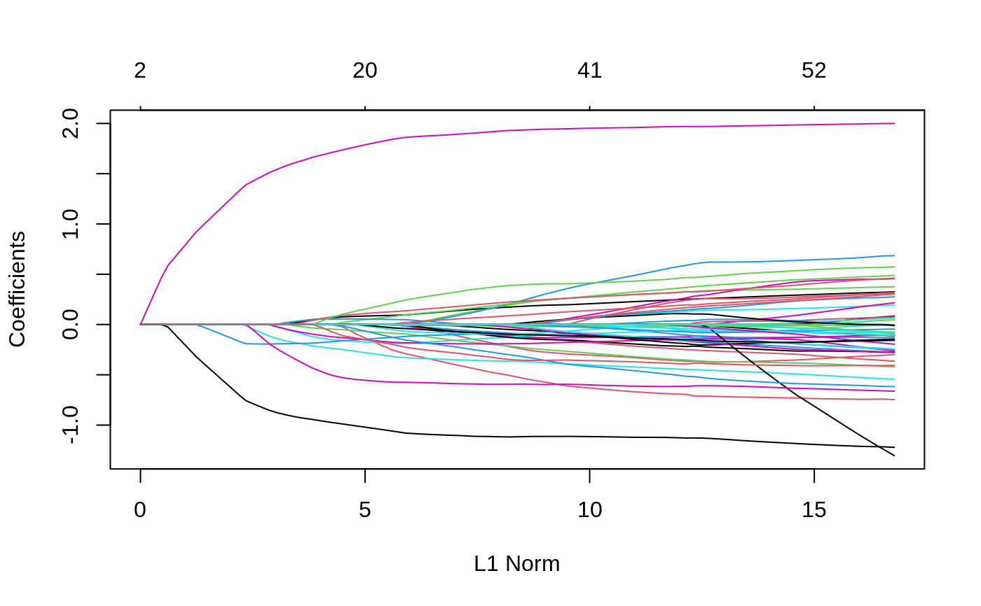
Examples

data(admixed)
fitlmm <- ggmix(x = admixed$xtrain, y = admixed$ytrain,
                kinship = admixed$kin_train,
                estimation = "full")
gicfit <- gic(fitlmm)
coef(gicfit, type = "nonzero")
#>                       1
#> (Intercept) -0.03660806
#> X302        -0.17607392
#> X524         1.34951500
#> X538        -0.72052613
#> eta          0.99000000
#> sigma2       1.60476289
predict(gicfit, newx = admixed$xtest)[1:5,,drop=FALSE]
#>                1
#> id26  2.31027410
#> id39  0.86922183
#> id45 -0.12814532
#> id52 -0.03660806
#> id53 -0.21268198
plot(gicfit)
plot(fitlmm)