21 Data Import and Export

This section is adapted from The Epidemiologist R Handbook¹²⁷

In this page we describe ways to locate, import, and export files:

• Use of the rio package to flexibly import() and export() many types of files
  
• Use of the here package to locate files relative to an R project root - to prevent complications from file paths that are specific to one computer
  
• Specific import scenarios, such as:
  • Specific Excel sheets
    
  • Messy headers and skipping rows
    
  • From Google sheets
    
  • From data posted to websites
    
  • With APIs
    
  • Importing the most recent file
    
• Manual data entry
  
• R-specific file types such as RDS and RData
  
• Exporting/saving files and plots

21.1 Overview

When you import a “dataset” into R, you are generally creating a new data frame object in your R environment and defining it as an imported file (e.g. Excel, CSV, TSV, RDS) that is located in your folder directories at a certain file path/address.

You can import/export many types of files, including those created by other statistical programs (SAS, STATA, SPSS). You can also connect to relational databases.

R even has its own data formats:

• An RDS file (.rds) stores a single R object such as a data frame. These are useful to store cleaned data, as they maintain R column classes. Read more in this section.
  
• An RData file (.Rdata) can be used to store multiple objects, or even a complete R workspace. Read more in this section.

21.2 The rio package

The R package we recommend is: rio. The name “rio” is an abbreviation of “R I/O” (input/output).

Its functions import() and export() can handle many different file types (e.g. .xlsx, .csv, .rds, .tsv). When you provide a file path to either of these functions (including the file extension like “.csv”), rio will read the extension and use the correct tool to import or export the file.

The alternative to using rio is to use functions from many other packages, each of which is specific to a type of file. For example, read.csv() (base R), read.xlsx() (openxlsx package), and write_csv() (readr pacakge), etc. These alternatives can be difficult to remember, whereas using import() and export() from rio is easy.

rio’s functions import() and export() use the appropriate package and function for a given file, based on its file extension. See the end of this page for a complete table of which packages/functions rio uses in the background. It can also be used to import STATA, SAS, and SPSS files, among dozens of other file types.

21.3 The here package

The package here and its function here() make it easy to tell R where to find and to save your files - in essence, it builds file paths.

Used in conjunction with an [R Project][projects], here allows you to describe the location of files in your R Project in relation to the R Project’s root directory (the top-level folder). This is useful when the R project may be shared or accessed by multiple people/computers. It prevents complications due to the unique file paths on different computers (e.g. "C:/Users/Laura/Documents..." by “starting” the file path in a place common to all users (the R Project root). See Chapter 18 for a reminder about R Projects.

This is how here() works within an R Project:

• When the here package is first loaded within the R Project, it places a small file called “.here” in the root folder of your R project as a “benchmark” or “anchor”
  
• In your scripts, to reference a file in the R project’s sub-folders, you use the function here() to build the file path in relation to that anchor
• To build the file path, write the names of folders beyond the root, within quotes, separated by commas, finally ending with the file name and file extension as shown below
  
• here() file paths can be used for both importing and exporting

For example, below, the function import() is being provided a file path constructed with here().

linelist <- rio::import(here::here("data", "linelists", "ebola_linelist.xlsx"))

The command here::here("data", "linelists", "ebola_linelist.xlsx") is actually providing the full file path that is unique to the user’s computer:

"C:/Users/Laura/Documents/my_R_project/data/linelists/ebola_linelist.xlsx"

The beauty is that the R command using here() can be successfully run on any computer accessing the R project.

If you are unsure where the “.here” root is set to, run the function here() with empty parentheses. Read more about the here package at this link.

21.4 File paths

When importing or exporting data, you must provide a file path. You can do this one of three ways:

1. Recommended: provide a “relative” file path with the here package
   
2. Provide the “full” / “absolute” file path
   
3. Manual file selection

21.4.1 “Relative” file paths

In R, “relative” file paths consist of the file path relative to the root of an R project. They allow for more simple file paths that can work on different computers (e.g. if the R project is on a shared drive or is sent by email). As described above, relative file paths are facilitated by use of the here package.

An example of a relative file path constructed with here() is below. In Figure 21.1 I show an example of a directory on my computer, with the epib607.Rproj file. This is referred to as the root directory of your project. All file paths will be relative to this directory. In this example the root directory is /home/sahir/git_repositories/epib607.

knitr::include_graphics(here::here("inst","figures","proj1.png"))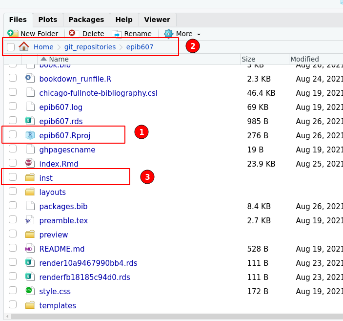

Figure 21.1: The files in my epib607 R project. (1) The R project file - this indicates that I have indeed created an R project called epib607. The .Rporj file is always found in the root directory. (2) The path of the directory as would be seen in a file management application such as Finder (on a mac) or Windows Explorer. (3) A directory that contains data.

The data I want to load is in a sub-folder called “inst” and within that, a subfolder “data”, in which there is the .rds file of interest as shown in Figure 21.2

knitr::include_graphics(here::here("inst","figures","proj2.png"))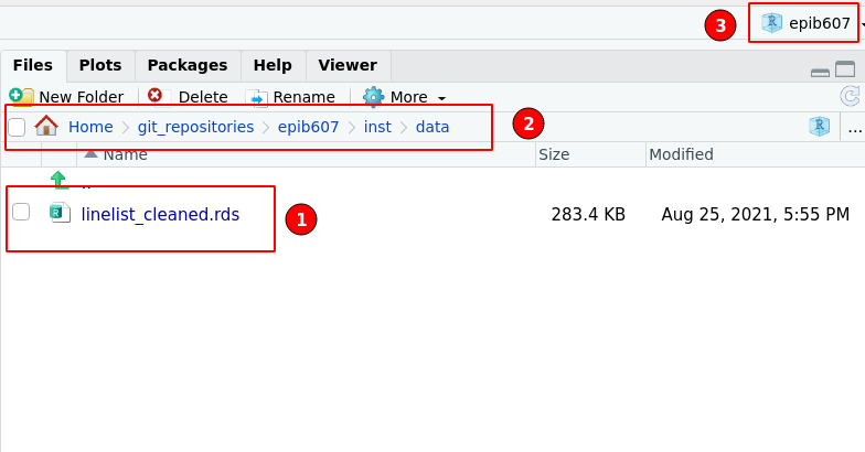

Figure 21.2: The sub-folder containing the data I want to load. (1) linelist_cleaned.rds is the data file. (2) The path of the directory as would be seen in a file management application such as Finder (on a mac) or Windows Explorer. (3) Indicator that I am indeed in the RStudio project called epib607.

To load the data, I simply call the rio::import() function. This function requires the location of the data file. I use the here::here() to locate the datafile:

linelist <- rio::import(here::here("inst","data", "linelist_cleaned.rds"))

21.4.2 “Absolute” file paths

Absolute or “full” file paths can be provided to functions like import() but they are “fragile” as they are unique to the user’s specific computer and therefore not recommended.

Below is an example of an absolute file path, where in Laura’s computer there is a folder “analysis”, a sub-folder “data” and within that a sub-folder “linelists”, in which there is the .xlsx file of interest.

linelist <- rio::import("/home/sahir/git_repositories/epib607/inst/data/linelist_cleaned.rds")

A few things to note about absolute file paths:

• Avoid using absolute file paths as they will break if the script is run on a different computer
• Use forward slashes (/), as in the example above (note: this is NOT the default for Windows file paths)
  
• File paths that begin with double slashes (e.g. “//…”) will likely not be recognized by R and will produce an error. Consider moving your work to a “named” or “lettered” drive that begins with a letter (e.g. “J:” or “C:”).

One scenario where absolute file paths may be appropriate is when you want to import a file from a shared drive that has the same full file path for all users.

TIP: To quickly convert all \ to /, highlight the code of interest, use Ctrl+f (in Windows), check the option box for “In selection”, and then use the replace functionality to convert them.

21.5 Import data from Excel

By default, if you provide an Excel workbook (.xlsx) to rio::import(), the workbook’s first sheet will be imported. If you want to import a specific sheet, include the sheet name to the which = argument. For example:

my_data <- rio::import("my_excel_file.xlsx", which = "Sheetname")

If using the here() method to provide a relative pathway to import(), you can still indicate a specific sheet by adding the which = argument after the closing parentheses of the here() function.

# Demonstration: importing a specific Excel sheet when using relative pathways with the 'here' package
linelist_raw <- rio::import(here::here("data", "linelist.xlsx"), which = "Sheet1")  

21.6 Missing values

You may want to designate which value(s) in your dataset should be considered as missing. The value in R for missing data is NA, but perhaps the dataset you want to import uses 99, “Missing”, or just empty character space "" instead.

Use the na = argument for rio::import() and provide the value(s) within quotes (even if they are numbers). You can specify multiple values by including them within a vector, using c() as shown below.

Here, the value “99” in the imported dataset is considered missing and converted to NA in R.

linelist <- rio::import(here::here("data", "my_linelist.xlsx"), na = "99")

Here, any of the values “Missing”, "" (empty cell), or " " (single space) in the imported dataset are converted to NA in R.

linelist <- rio::import(here::here("data", "my_linelist.csv"), na = c("Missing", "", " "))

21.7 Skip rows

Sometimes, you may want to avoid importing a row of data. You can do this with the argument skip = if using import() from rio on a .xlsx or .csv file. Provide the number of rows you want to skip.

linelist_raw <- rio::import("linelist_raw.xlsx", skip = 1)  # does not import header row

Unfortunately skip = only accepts one integer value, not a range (e.g. “2:10” does not work).

21.8 Import from Google sheets

You can import data from an online Google spreadsheet with the googlesheet4 package and by authenticating your access to the spreadsheet.

pacman::p_load("googlesheets4")

Below, a demo Google sheet is imported and saved. This command may prompt confirmation of authentification of your Google account. Follow prompts and pop-ups in your internet browser to grant Tidyverse API packages permissions to edit, create, and delete your spreadsheets in Google Drive.

The sheet below is “viewable for anyone with the link” and you can try to import it.

Gsheets_demo <- read_sheet("https://docs.google.com/spreadsheets/d/1scgtzkVLLHAe5a6_eFQEwkZcc14yFUx1KgOMZ4AKUfY/edit#gid=0")

The sheet can also be imported using only the sheet ID, a shorter part of the URL:

Gsheets_demo <- read_sheet("1scgtzkVLLHAe5a6_eFQEwkZcc14yFUx1KgOMZ4AKUfY")

Another package, googledrive offers useful functions for writing, editing, and deleting Google sheets. For example, using the gs4_create() and sheet_write() functions found in this package.

Here are some other helpful online tutorials:
basic Google sheets importing tutorial
more detailed tutorial
interaction between the googlesheets4 and tidyverse

21.9 Import from Github

Importing data directly from Github into R can be very easy or can require a few steps - depending on the file type. Below are some approaches:

21.9.1 CSV files

It can be easy to import a .csv file directly from Github into R with an R command.

1. Go to the Github repo https://github.com/sahirbhatnagar/knitr-tutorial, locate the file 001-motivating-example/fat-data.csv, and click on it
   
2. Click on the “Raw” button (you will then see the “raw” csv data, as shown below)
   
3. Copy the URL (web address)
   
4. Place the URL in quotes within the import() R command

Figure 14.4: Getting the link to data in .csv format from a GitHub repository.

Once you’ve copied the URL address of the file, you can use the rio::import function as follows:

df <- rio::import("https://raw.githubusercontent.com/sahirbhatnagar/knitr-tutorial/master/001-motivating-example/fat-data.csv")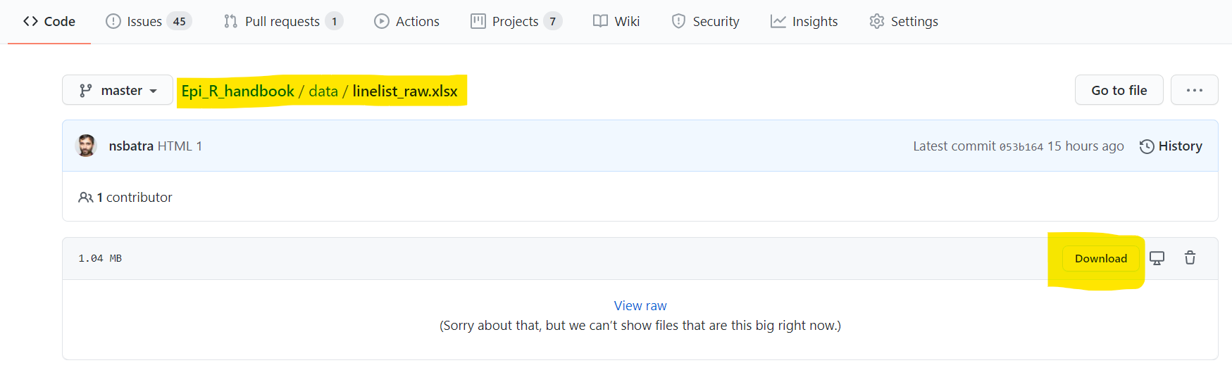

21.9.2 XLSX files

You may not be able to view the “Raw” data for some files (e.g. .xlsx, .rds, .nwk, .shp)

1. Go to the Github repo, locate the file of interest, and click on it
   
2. Click the “Download” button, as shown below
   
3. Save the file on your computer, and import it into R

21.10 Manual data entry

21.10.1 Entry by rows

Use the tribble function from the tibble package from the tidyverse (online tibble reference).

Note how column headers start with a tilde (~). Also note that each column must contain only one class of data (character, numeric, etc.). You can use tabs, spacing, and new rows to make the data entry more intuitive and readable. Spaces do not matter between values, but each row is represented by a new line of code. For example:

# create the dataset manually by row
manual_entry_rows <- tibble::tribble(
  ~colA, ~colB,
  "a",   1,
  "b",   2,
  "c",   3
  )

And now we display the new dataset:

21.10.2 Entry by columns

Since a data frame consists of vectors (vertical columns), the base approach to manual dataframe creation in R expects you to define each column and then bind them together. This can be counter-intuitive in epidemiology, as we usually think about our data in rows (as above).

# define each vector (vertical column) separately, each with its own name
PatientID <- c(235, 452, 778, 111)
Treatment <- c("Yes", "No", "Yes", "Yes")
Death     <- c(1, 0, 1, 0)

CAUTION: All vectors must be the same length (same number of values).

The vectors can then be bound together using the function data.frame():

# combine the columns into a data frame, by referencing the vector names
manual_entry_cols <- data.frame(PatientID, Treatment, Death)

And now we display the new dataset:

21.10.3 Pasting from clipboard

If you copy data from elsewhere and have it on your clipboard, you can try using the datapasta R package which allows you to import as a data frame as shown in Figure 21.3:

Figure 21.3: Copying data to your clipboard and pasting as a data frame in R.

21.11 Export

21.11.1 With rio package

With rio, you can use the rio::export() function in a very similar way to rio::import(). First give the name of the R object you want to save (e.g. linelist) and then in quotes put the file path where you want to save the file, including the desired file name and file extension. For example:

This saves the data frame linelist as an Excel workbook to the working directory (R Project root folder):

rio::export(linelist, "my_linelist.xlsx") # will save to working directory

You could save the same data frame as a csv file by changing the extension. For example, we also save it to a file path constructed with here():

rio::export(linelist, here::here("data", "clean", "my_linelist.csv"))

21.12 RDS files

Along with .csv, .xlsx, etc, you can also export/save R data frames as .rds files. This is a file format specific to R, and is very useful if you know you will work with the exported data again in R.

The classes of columns are stored, so you don’t have do to cleaning again when it is imported (with an Excel or even a CSV file this can be a headache!). It is also a smaller file, which is useful for export and import if your dataset is large.

rio::export(linelist, here::here("data", "clean", "my_linelist.rds"))

21.13 Rdata files and lists

.Rdata files can store multiple R objects - for example multiple data frames, model results, lists, etc. This can be very useful to consolidate or share a lot of your data for a given project.

In the below example, multiple R objects are stored within the exported file “my_objects.Rdata”:

rio::export(my_list, my_dataframe, my_vector, "my_objects.Rdata")

Note: if you are trying to import a list, use rio::import_list() to import it with the complete original structure and contents.

rio::import_list("my_list.Rdata")

21.14 Saving plots

Instructions on how to save plots, such as those created by ggplot(), are discussed in depth in the [ggplot basics] page.

In brief, run ggsave("my_plot_filepath_and_name.png") after printing your plot. You can either provide a saved plot object to the plot = argument, or only specify the destination file path (with file extension) to save the most recently-displayed plot. You can also control the width =, height =, units =, and dpi =.

How to save a network graph, such as a transmission tree, is addressed in the page on [Transmission chains].

21.15 Resources

The R Data Import/Export Manual
R 4 Data Science chapter on data import
ggsave() documentation

Below is a table, taken from the rio online vignette. For each type of data it shows: the expected file extension, the package rio uses to import or export the data, and whether this functionality is included in the default installed version of rio.

Format	Typical Extension	Import Package	Export Package	Installed by Default
Comma-separated data	.csv	data.table fread()	data.table	Yes
Pipe-separated data	.psv	data.table fread()	data.table	Yes
Tab-separated data	.tsv	data.table fread()	data.table	Yes
SAS	.sas7bdat	haven	haven	Yes
SPSS	.sav	haven	haven	Yes
Stata	.dta	haven	haven	Yes
SAS	XPORT	.xpt	haven	haven
SPSS Portable	.por	haven		Yes
Excel	.xls	readxl		Yes
Excel	.xlsx	readxl	openxlsx	Yes
R syntax	.R	base	base	Yes
Saved R objects	.RData, .rda	base	base	Yes
Serialized R objects	.rds	base	base	Yes
Epiinfo	.rec	foreign		Yes
Minitab	.mtp	foreign		Yes
Systat	.syd	foreign		Yes
“XBASE”	database files	.dbf	foreign	foreign
Weka Attribute-Relation File Format	.arff	foreign	foreign	Yes
Data Interchange Format	.dif	utils		Yes
Fortran data	no recognized extension	utils		Yes
Fixed-width format data	.fwf	utils	utils	Yes
gzip comma-separated data	.csv.gz	utils	utils	Yes
CSVY (CSV + YAML metadata header)	.csvy	csvy	csvy	No
EViews	.wf1	hexView		No
Feather R/Python interchange format	.feather	feather	feather	No
Fast Storage	.fst	fst	fst	No
JSON	.json	jsonlite	jsonlite	No
Matlab	.mat	rmatio	rmatio	No
OpenDocument Spreadsheet	.ods	readODS	readODS	No
HTML Tables	.html	xml2	xml2	No
Shallow XML documents	.xml	xml2	xml2	No
YAML	.yml	yaml	yaml	No
Clipboard default is tsv		clipr	clipr	No