Chapter 3 Discrete Random Variables and Probability Distributions
Introduction
In Chapter 2, we discussed the probability model as the central object of study in the theory of probability. This required defining a probability measure \(P\) on a class of subsets of the sample space \(\Omega\). For example, for an experiment with possible sample outcomes denoted by the \(\Omega\), an \(E\) was defined as any collection of sample outcomes, that is, any subset of the set \(\Omega\).
\[ \begin{array}{ccll} \text{EXPERIMENT} & \longrightarrow \text{SAMPLE OUTCOMES} & \longrightarrow \text{EVENTS} & \longrightarrow \text{PROBABILITIES} \\ & \Omega=\left\{ s_{1},s_{2},...\right\} & \longrightarrow E\subseteq S & \longrightarrow P(E) \end{array} \]
In this framework, it is necessary to consider each experiment with its associated sample space separately - the nature of sample space \(\Omega\) is typically different for different experiments.
Example 3.1 (Rainy days) Count the number of days in February which have zero precipitation.
\[ \Omega = \left\{ 0,1,2,\ldots,28\right\} \]
Let \(E_{i}\) = \(i\) days have zero precipitation. \(E_{0},\ldots,E_{28}\) partition \(\Omega\).
Example 3.2 (Footbal Match) Count the number of goals in a football match.
\[ \Omega = \left\{ 0,1,2,3,\ldots \right\} \]
Let \(E_{i}\) = \(i\) goals in the match. \(E_{0},E_{1},E_{2},\ldots\) partition \(\Omega\)In both of these examples, we need a formula to specify each
\[ P(E_{i}) = p_{i} \]
Example 3.3 (Operating Temperature) Measure the operating temperature of an experimental process.
\[ \Omega = \left\{ x: x > T_{min} \right\} \]
Here it is difficult to express
\[ P(``\textrm{Measurement is }x") \]
but possible to think about
\[ P (``\textrm{Measurement is }\leq x")=F(x) \]
and now we seek a formula for \(F(x)\) which is a simpler way of presenting a particular probability assignment.
This chapter is concerned with the definitions of random variables, distribution functions \(F(x)\), probability/density functions \(f(x)\), and the development of the concepts necessary for carrying out calculations for a probability model using these entities (Evans and Rosenthal 2004).
The concept of a random variable allows us to pass from the experimental outcomes themselves to a numerical function of the outcomes. There are two fundamentally different types of random variables (Devore and Berk 2011):
- discrete random variables
- continuous random variables
In this chapter, we examine the basic properties and discuss the most important examples of discrete variables. Chapter 4 focuses on continuous random variables.
3.1 Random Variables
A general notation useful for all such examples can be obtained by considering a sample space that is equivalent to \(\Omega\) for a general experiment, but whose form is more familiar.
Definition 3.1 (Random Variable) A random variable \(X\) on \(\Omega\) is a function from the sample space \(\Omega\) to the set \(\mathbb{R}\) of all real numbers denoted by
\[ X : \Omega \rightarrow \mathbb{R} \]
Let \(R_X\) denote the range of \(X\).
\(X\) is called a discrete random variable if \(R_X\) is a countable set.
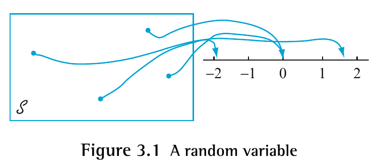
Random variables are customarily denoted by uppercase letters, such as \(X\) and \(Y\), lowercase letters to represent some particular value of the corresponding random variable. The notation \(X(s) = x\) means that \(x\) is the value associated with the outcome \(s\) by the rv \(X\).
Example 3.4 (Coin Toss) Suppose a coin is tossed three times. Let \(X\) be the number of heads observed. The sample space is
\[ \Omega = \left\lbrace \underbrace{HHT}_{3},\underbrace{HHT}_{2},\underbrace{HTH}_{2},\underbrace{HTT}_{1}, \underbrace{THH}_{2}, \underbrace{THT}_{1}, \underbrace{TTH}_{1}, \underbrace{TTT}_{0} \right\rbrace \]
That is, we have \(X(HHH) = 3\), \(X(HHT) = 2\), \(X(HTH) = 2\), and so on. Hence \(R_X = \left\lbrace 0,1,2,3 \right\rbrace\)We now present several further examples. The point is, we can define random variables any way we like, as long as they are functions from the sample space to \(\mathbb{R}\).
Example 3.6 (A Very Simple Random Variable 2) For the case \(\Omega = \left\lbrace \textrm{rain, snow, clear} \right\rbrace\), we might define a second random variable \(Y\) by saying that \(Y = 0\) if it rains, \(Y = -1/2\) if it snows, and \(Y = 7/8\) if it is clear. That is \(Y(rain) = 0\), \(Y(snow) = 1/2\), and \(Y(rain) = 7/8\).
Example 3.7 (A Very Simple Random Variable 3) If the sample space corresponds to flipping three different coins, then we could let \(X\) be the total number of heads showing, let \(Y\) be the total number of tails showing, let \(Z = 0\) if there is exactly one head, and otherwise \(Z = 17\).
Example 3.8 (Constants as Random Variables) As a special case, every constant value \(c\) is also a random variable, by saying that \(c(s) = c\) for all \(s \in \Omega\). Thus, 5 is a random variable, as is 3 or −21.6.
Example 3.9 (Indicator Functions) If \(A\) is any event, then we can define the indicator function of \(A\), written \(I_A\), to be the random variable
\[I_A(s) = \begin{cases} 1 & s \in A \\ 0 & s \notin A \end{cases} \]
Suppose \(X\) is a random variable. We know that different states \(s\) occur with different probabilities. It follows that \(X(s)\) also takes different values with different probabilities. These probabilities are called the distribution of \(X\); we consider them next.
3.2 Probability Distributions for Discrete Random Variables
Because random variables are defined to be functions of the outcome \(s\), and because the outcome \(s\) is assumed to be random (i.e., to take on different values with different probabilities), it follows that the value of a random variable will itself be random (as the name implies).
Specifically, if \(X\) is a random variable, then what is the probability that \(X\) will equal some particular value \(x\)? Well, \(X = x\) precisely when the outcome \(s\) is chosen such that \(X(s) = x\).
3.3 Expected Values of Discrete Random Variables
3.4 Moments and Moment Generating Functions
3.5 The Binomial Probability Distribution
3.6 The Poisson Probability Distribution
References
Evans, Michael J, and Jeffrey S Rosenthal. 2004. Probability and Statistics: The Science of Uncertainty. Macmillan.
Devore, Jay L, and Kenneth N Berk. 2011. Modern Mathematical Statistics with Applications. Springer Science & Business Media.