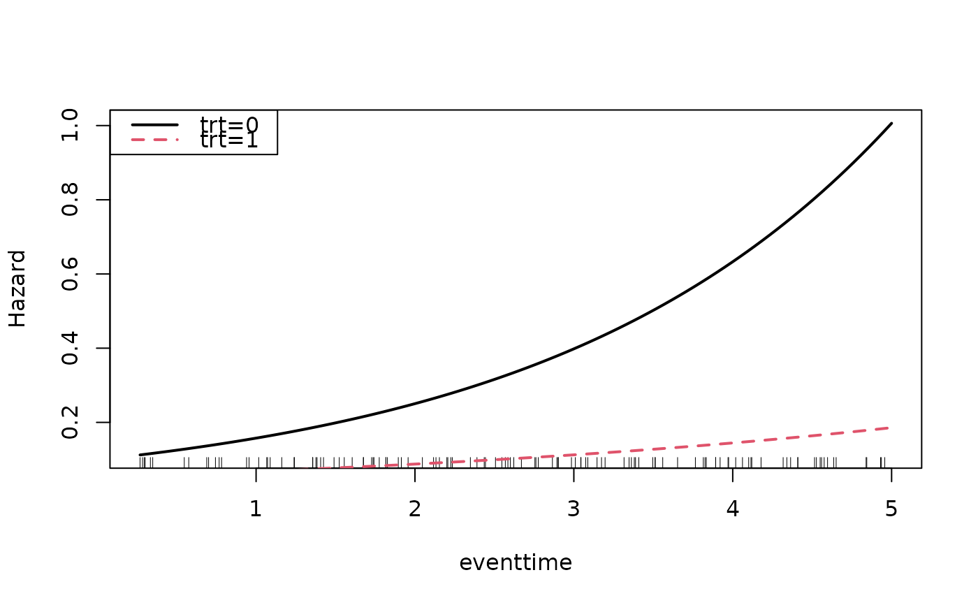
Visualize estimated hazard curves as a function of time with
confidence intervals. This function takes as input, the result from the
fitSmoothHazard() function. The user can also specify a
sequence of times at which to estimate the hazard function. These plots are
useful to visualize the non-proportional hazards, i.e., time dependent
interactions with a covariate.
Arguments
- object
Fitted object of class
glm,gam,cv.glmnetorgbm. This is the result from thefitSmoothHazard()function.- newdata
A data frame in which to look for variables with which to predict. This is required and must contain all the variables used in the model. Only one covariate profile can be used. If more than one row is provided, only the first row will be used.
- type
Type of plot. Currently, only "hazard" has been implemented. Default: c("hazard")
- xlab
x-axis label. Default: the name of the time variable from the fitted
object.- breaks
Number of points at which to estimate the hazard. This argument is only used if argument
times=NULL. This function will calculate a sequence of times between the minimum and maximum of observed event times. Default: 100.- ci.lvl
Confidence level. Must be in (0,1), Default: 0.95
- ylab
y-axis label. Default: NULL which means the function will put sensible defaults.
- line.col
Line color, Default: 1. See
graphics::par()for details.- ci.col
Confidence band color. Only used if argument
ci=TRUE, Default: 'grey'- lty
Line type. See
graphics::par()for details, Default: par("lty")- add
Logical; if TRUE add to an already existing plot; Default: FALSE
- ci
Logical; if TRUE confidence bands are calculated. Only available for
family="glm"andfamily="gam", Default: !add- rug
Logical. Adds a rug representation (1-d plot) of the event times (only for
status=1), Default: !add- s
Value of the penalty parameter lambda at which predictions are required (for class
cv.glmnetonly). Only the first entry will be used if more than one numeric value is provided, Default: c("lambda.1se", "lambda.min")- times
Vector of numeric values at which the hazard should be calculated. Default: NULL which means this function will use the minimum and maximum of observed event times with the
breaksargument.- ...
further arguments passed to
graphics::matplot()
Value
a plot of the hazard function and a data.frame of original data used
in the fitting along with the data used to create the plots including
predictedhazard which is the predicted hazard for a given covariate
pattern and time predictedloghazard is the predicted hazard on the log
scale. lowerbound and upperbound are the lower and upper confidence
interval bounds on the hazard scale (i.e. used to plot the confidence
bands). standarderror is the standard error of the log hazard (only if
family="glm" or family="gam")
Details
This is an earlier version of a function to plot hazards. We
recommend instead using the plot method for objects returned by
fitSmoothHazard(). See plot.singleEventCB().
See also
Examples
data("simdat")
mod_cb <- fitSmoothHazard(status ~ trt * eventtime,
                                    time = "eventtime",
                                    data = simdat[1:200,],
                                    ratio = 1,
                                    family = "glm")

results0 <- hazardPlot(object = mod_cb, newdata = data.frame(trt = 0),
           ci.lvl = 0.95, ci = FALSE, lty = 1, line.col = 1, lwd = 2)
head(results0)
#>     trt eventtime offset predictedloghazard predictedhazard
#> 1     0 0.2695865      0          -2.186588       0.1122993
#> 1.1   0 0.3173684      0          -2.164438       0.1148144
#> 1.2   0 0.3651504      0          -2.142289       0.1173859
#> 1.3   0 0.4129323      0          -2.120139       0.1200149
#> 1.4   0 0.4607143      0          -2.097989       0.1227029
#> 1.5   0 0.5084963      0          -2.075840       0.1254510
hazardPlot(object = mod_cb, newdata = data.frame(trt = 1), ci = FALSE,
           ci.lvl = 0.95, add = TRUE, lty = 2, line.col = 2, lwd = 2)
legend("topleft", c("trt=0","trt=1"),lty=1:2,col=1:2,bty="y", lwd = 2)
