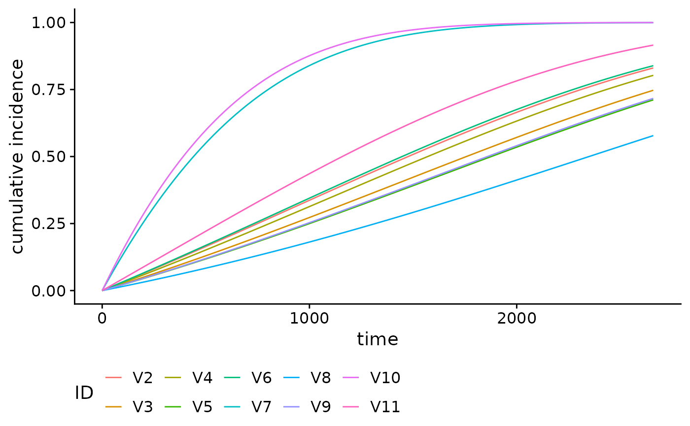
Plot Cumulative Incidence and Survival Curves

Sahir Rai Bhatnagar

2024-08-17

Introduction

In this short vignette, we will introduce the plot method for absoluteRisk objects. This method allows you to plot cumulative incidence (CI) or survival curves as a function of time and a given covariate profile. More specifically, the cumulative incidence is given by:

$$CI(x, t) = 1 - exp\left[ - \int_0^t h(x, u) \textrm{d}u \right]$$ where \( h(x, t) \) is the hazard function, \( t \) denotes the numerical value (number of units) of a point in prognostic/prospective time and \( x \) is the realization of the vector \( X \) of variates based on the patient’s profile and intervention (if any). And the survival function is given by $$S(x, t) = 1 - CI(x,t) = exp\left[ - \int_0^t h(x, u) \textrm{d}u \right]$$

Analysis of the brcancer dataset

To illustrate hazard function plots, we will use the breast cancer dataset which contains the observations of 686 women taken from the TH.data package. This dataset is also available from the casebase package. In the following, we will show the CI curve for several covariate profiles.

library(casebase)
#> See example usage at http://sahirbhatnagar.com/casebase/
library(survival)
library(ggplot2)


data("brcancer")
mod_cb_glm <- fitSmoothHazard(cens ~ estrec*log(time) + 
                                  horTh + 
                                  age + 
                                  menostat + 
                                  tsize + 
                                  tgrade + 
                                  pnodes + 
                                  progrec,
                              data = brcancer,
                              time = "time", ratio = 10)

summary(mod_cb_glm)

Plotting Cumulative Incidence Curves

We can use the plot method for objects of class absRiskCB, which is returned by the absoluteRisk function, to plot cumulative incidence curves. For example, suppose we want to compare the cumulative incidence curves of the 1st and 50th individuals in the brcancer dataset. We first call the absoluteRisk function and specify the newdata argument. Note that since time is missing, the risk estimate is calculated at the observed failure times.

smooth_risk_brcancer <- absoluteRisk(object = mod_cb_glm, 
                                     newdata = brcancer[c(1,50),])

class(smooth_risk_brcancer)
plot(smooth_risk_brcancer)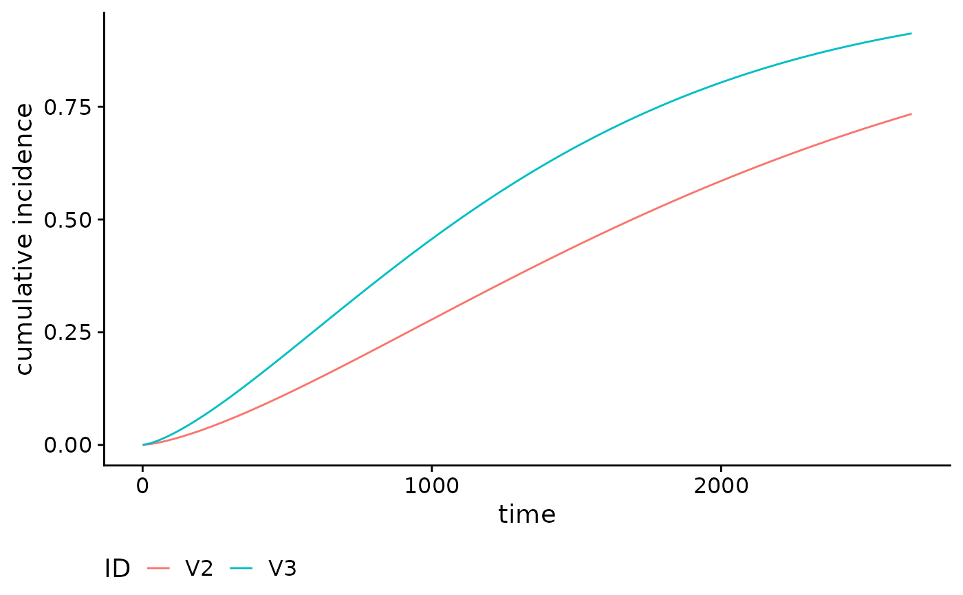

These curves can be further customized. For example, suppose we want to change the legend title and legend keys:

plot(smooth_risk_brcancer, 
     id.names = c("Covariate Profile 1","Covariate Profile 50"), 
     legend.title = "Type", 
     xlab = "time (days)", 
     ylab = "Cumulative Incidence (%)")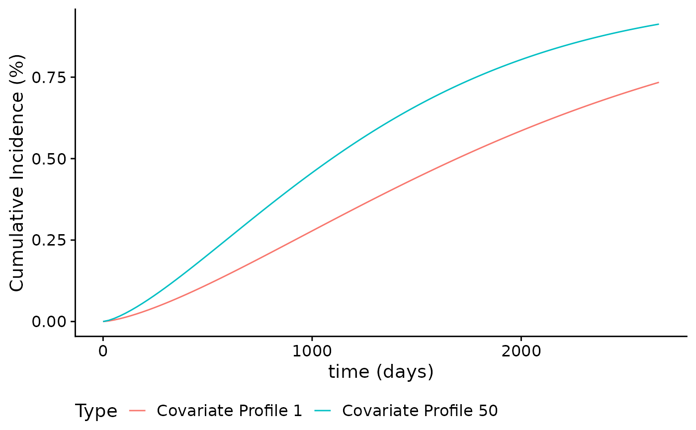 

The call to plot on a absRiskCB object returns a ggplot2 object, and therefore can be used downstream with other ggplot2 functions. For example, suppose we want to change the theme:

plot(smooth_risk_brcancer, 
     id.names = c("Covariate Profile 1","Covariate Profile 50"), 
     legend.title = "Type", 
     xlab = "time (days)", 
     ylab = "Cumulative Incidence (%)") + ggplot2::theme_linedraw()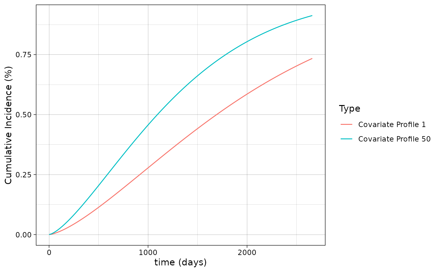 

Using graphics::matplot

By default, the plot method uses ggplot2 to produce the curves. Alternatively, you can use graphics::matplot by specifying gg = FALSE. This option is particularly useful if you want to add the cumulative incidence curve to an existing plot, e.g., adding the adjusted smooth curve to a Kaplan-Meier curve. In this example, we calculate the cumulative incidence for a typical individual in the dataset:

cols <- c("#8E063B","#023FA5")

smooth_risk_typical <- absoluteRisk(object = mod_cb_glm, newdata = "typical")
y <- with(brcancer, survival::Surv(time, cens))
plot(y, fun = "event", conf.int = F, col = cols[1], lwd = 2)
plot(smooth_risk_typical, add = TRUE, col = cols[2], lwd = 2, gg = FALSE)
legend("bottomright", 
       legend = c("Kaplan-Meier", "casebase"), 
       col = cols,
       lty = 1,
       lwd = 2,
       bg = "gray90")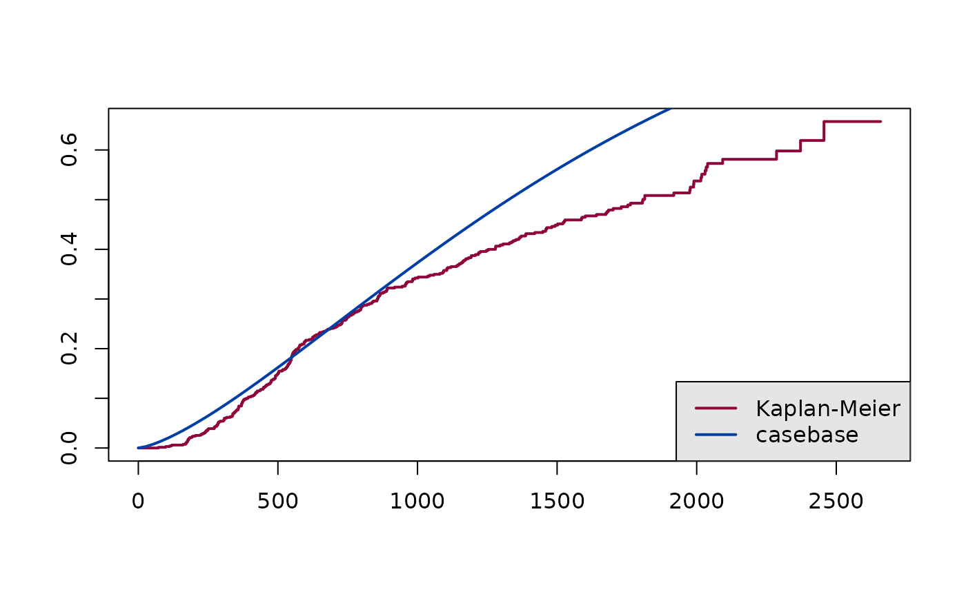

Survival Curves

We can also easily calculate and plot survival curves by specifying type = 'survival' in the call to absoluteRisk. The corresponding call to plot is the same as with cumulative incidence curves:

smooth_surv_brcancer <- absoluteRisk(object = mod_cb_glm, 
                                     newdata = brcancer[c(1,50),],
                                     type = "survival")

plot(smooth_surv_brcancer)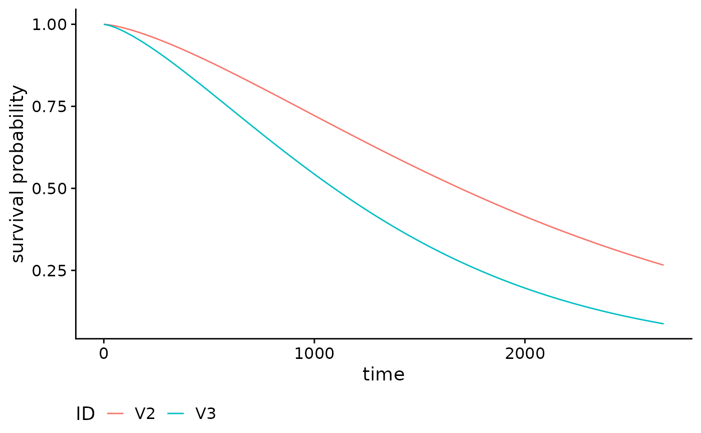

Other families

glmnet

We can also plot cumulative incidence curves for other families. For example, using the family = "glmnet", we can plot the cumulative incidence curves for the first 10 individuals in the brcancer dataset, using the tuning parameter which minimizes the 10-fold cross-validation error ($\lambda_{min}$):

mod_cb_glmnet <- fitSmoothHazard(cens ~ estrec*time + 
                                     horTh + 
                                     age + 
                                     menostat + 
                                     tsize + 
                                     tgrade + 
                                     pnodes + 
                                     progrec,
                                 data = brcancer,
                                 time = "time", 
                                 ratio = 1, 
                                 family = "glmnet")

smooth_risk_glmnet <- absoluteRisk(object = mod_cb_glmnet, 
                                   newdata = brcancer[1:10,], 
                                   s = "lambda.min")
plot(smooth_risk_glmnet)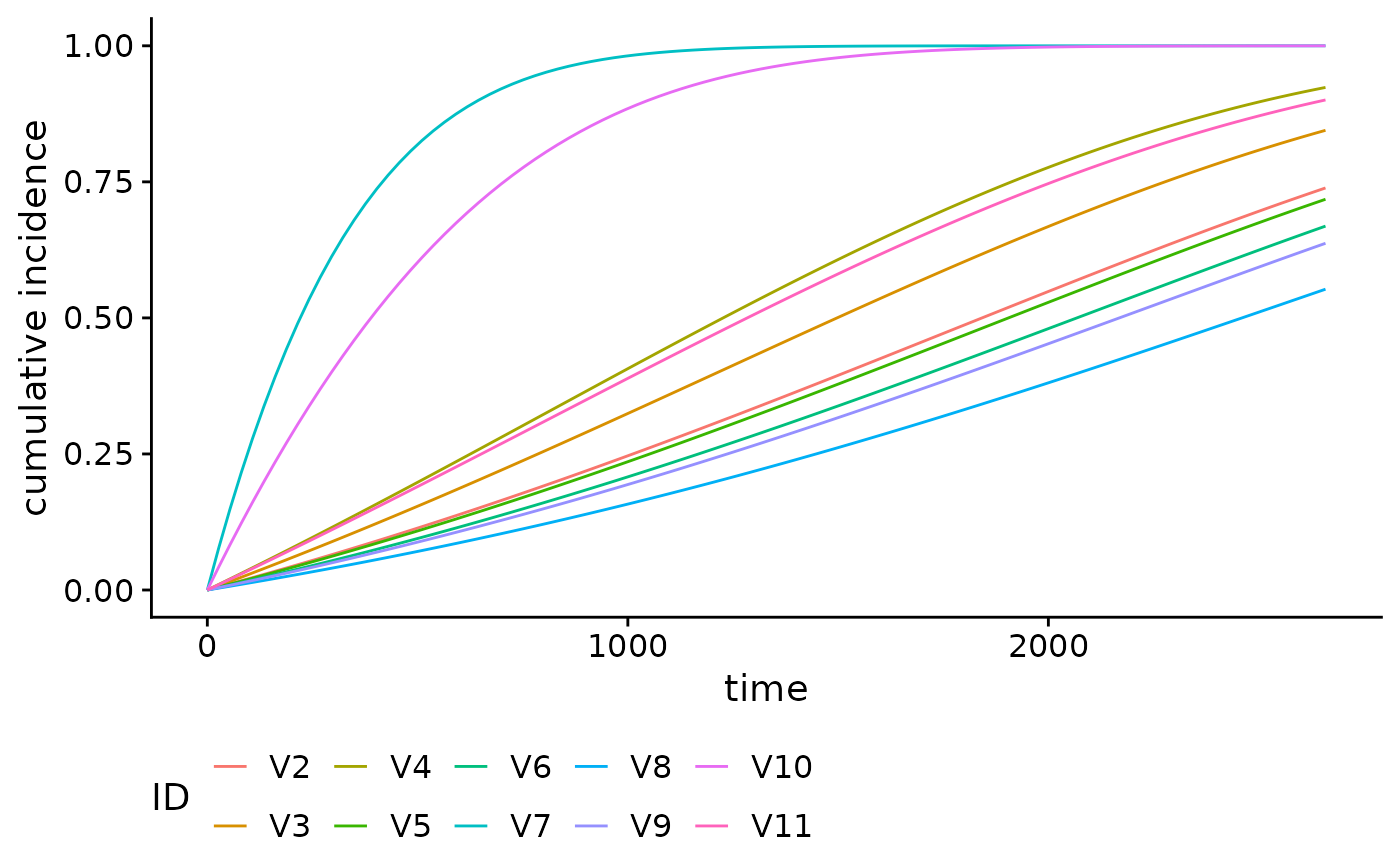

gam

Here we produce the same plot but for family = "gam" for generalised additive models.

mod_cb_gam <- fitSmoothHazard(cens ~ estrec + time + 
                                     horTh + 
                                     age + 
                                     menostat + 
                                     tsize + 
                                     tgrade + 
                                     pnodes + 
                                     progrec,
                                 data = brcancer,
                                 time = "time", 
                                 ratio = 1, 
                                 family = "gam")

smooth_risk_gam <- absoluteRisk(object = mod_cb_gam, 
                                newdata = brcancer[1:10,])
plot(smooth_risk_gam)

Session information