Data on the men in the European Randomized Study of Prostate Cancer Screening
Source:R/data.R
ERSPC.RdThis data set lists the individual observations for 159,893 men in the core age group between the ages of 55 and 69 years at entry.
ERSPCFormat
A data frame with 159,893 observations on the following 3 variables:
- ScrArm
Whether in Screening Arm (1) or non-Screening arm (0) (
numeric)- Follow.Up.Time
The time, measured in years from randomization, at which follow-up was terminated
- DeadOfPrCa
Whether follow-up was terminated by Death from Prostate Cancer (1) or by death from other causes, or administratively (0)
Source
The individual censored values were recovered by James Hanley from the Postcript code that the NEJM article (Schroder et al., 2009) used to render Figure 2 (see Liu et al., 2014, for details). The uncensored values were more difficult to recover exactly, as the 'jumps' in the Nelson-Aalen plot are not as monotonic as first principles would imply. Thus, for each arm, the numbers of deaths in each 1-year time-bin were estimated from the differences in the cumulative incidence curves at years 1, 2, ... , applied to the numbers at risk within the time-interval. The death times were then distributed at random within each bin.
The interested reader can 'see' the large numbers of individual censored values by zooming in on the original pdf Figure, and watching the Figure being re-rendered, or by printing the graph and watching the printer 'pause' while it superimposes several thousand dots (censored values) onto the curve. Watching these is what prompted JH to look at what lay 'behind' the curve. The curve itself can be drawn using fewer than 1000 line segments, and unless on peers into the PostScript) the almost 160,000 dots generated by Stata are invisible.
Details
The men were recruited from seven European countries (centers). Each centre began recruitment at a different time, ranging from 1991 to 1998. The last entry was in December 2003. The uniform censoring date was December 31, 2006. The randomization ratio was 1:1 in six of the seven centres. In the seventh, Finland, the size of the screening group was fixed at 32,000 subjects. Because the whole birth cohort underwent randomization, this led to a ratio, for the screening group to the control group, of approximately 1 to 1.5, and to the non-screening arm being larger than the screening arm.
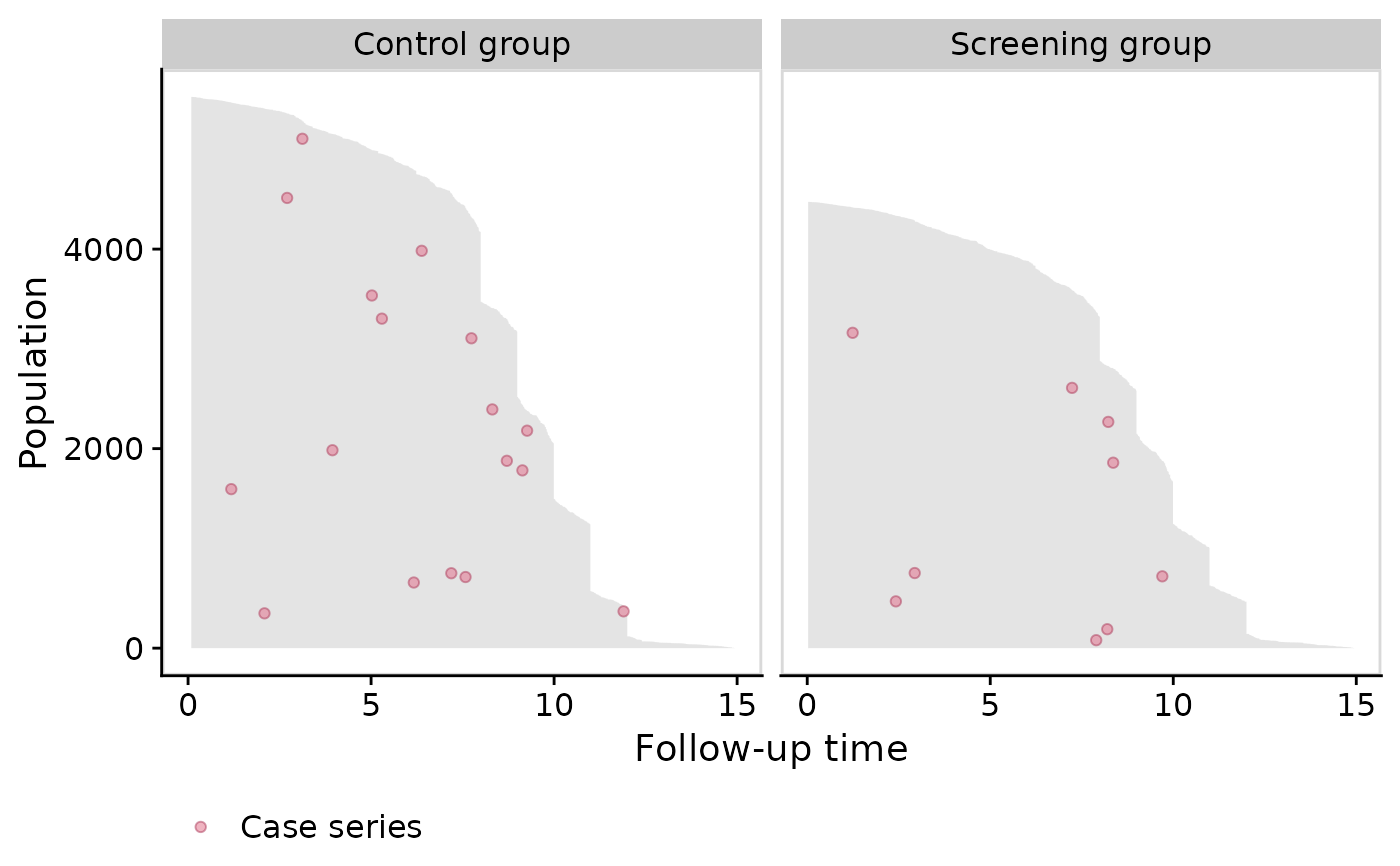
The randomization of the Finnish cohorts were carried out on January 1 of each of the 4 years 1996 to 1999. This, coupled with the uniform December 31 2006 censoring date, lead to large numbers of men with exactly 11, 10, 9 or 8 years of follow-up.
Tracked backwards in time (i.e. from right to left), the Population-Time plot shows the recruitment pattern from its beginning in 1991, and in particular the Jan 1 entries in successive years.
Tracked forwards in time (i.e. from left to right), the plot for the first 3 years shows attrition due entirely to death (mainly from other causes). Since the Swedish and Belgian centres were the last to close their recruitment - in December 2003 - the minimum potential follow-up is three years. Tracked further forwards in time (i.e. after year 3) the attrition is a combination of deaths and staggered entries.
References
Liu Z, Rich B, Hanley JA. Recovering the raw data behind a non-parametric survival curve. Systematic Reviews 2014; 3:151. doi:10.1186/2046-4053-3-151 .
Schroder FH, et al., for the ERSPC Investigators. Screening and Prostate-Cancer Mortality in a Randomized European Study. N Engl J Med 2009; 360:1320-8. doi:10.1056/NEJMoa0810084 .
