14 Binomial Random Variable

14.1 Objectives

Distributions of individual values take their shapes and spreads from the features of the setting, and thus do not follow any general laws. The shapes and the spreads of distributions of statistical summaries and parameter estimates made from aggregates of individual observations tend to be more regular and more predictable, and thus more law-abiding.

So, the specific objectives in this chapter are to truly understand

• the distinction between a natural and investigator-made distributions, and between observable and conceptual ones.

• why we should not automatically associate certain distributions with certain types of random variables

• why we need to understand the pre-requisites for random variables following the distributions they do

• why we rely so much on the Normal distribution, and why it is so ‘Central’ to statistical inference concerning parameters.

• why the pre-occupation with checking ‘Normality’ (Gaussian-ness) is misguided

• why Normality is not even relevant when the ‘variable’ is not ‘random’, and appears on the right hand side of a regression model.

• the few contexts where shape does matter

To get a full list of the named distributions available in R you can use the following command: help(Distributions)

14.2 Bernoulli

The simplest random variable is one that take just 2 possible values, such as YES/NO, MALE/FEMALE, 0/1, ON/OFF, POSITIVE/NEGATIVE, PRESENT/ABSENT, EXISTS/DOES NOT, etc.

This random variable \(Y\) is governed by just one parameter, namely the probability, \(\pi\), that it takes on the YES (or ‘1’) value. Of course you can reverse the scale, and speak about the probability of a NO (or ‘0’) result.

It is too bad that when Wikipedia, which has a unified way of showing the main features of statistical distributions, does not follow its own principles and show a graph of various versions of a Bernoulli distribution. So here is such a graph.

Figure 11.2: Various Bernoulli random variables/distributions. We continue our convention of using the letter Y (instead of X) as the generic name for a random variable. Moreover, in keeping with this view, all of the selected Bernoulli distributions are plotted with their 2 possible values shown on the vertical axis.

Please, when reading the Wikipedia entry, replace all instances of \(X\) and \(x\) by \(Y\) and \(y\). Note also that we will use \(\pi\) where Wikipedia, and some textbooks, use \(p\). As much as we can, we use Greek letters for parameters and Roman letters for their empirical (sample) counterparts. Also, to be consistent, if the random variable itslef is called \(Y\), then it makes sense to use \(y\) as the possible relaizations of it, rather than the illogical \(k\) that Wikipedia uses.]

In the sidebar, Wikipedia shows the probability mass function (pmf, the probabilities that go with the possible \(Y\) values) in two separate rows, but in the text the pmf is also shown more concisely, as (in our notation)

\[f(y) = \pi^y (1-\pi)^{1-y}, \ \ y = 0, 1.\] If we wish to align with how the R software names features of distributions, we might want to switch from \(f\) to \(d\). R uses \(d\) because it harmonizes with the probability \(d\)ensity function (pdf) notation that its uses for random variables on an interval scale, even though some statistical ‘purists’ see that as mixing terminology: they use the term probablility mass function for discrete random variables, and probablity density function for ones on an interval scale.

\[d_{Bernoulli}(y) = \pi^y (1-\pi)^{1-y}.\]

Sadly, Bernoulli does not get its own entry in R’s list of named distributions, presumably because it is a special case of a binomial distribution, one where \(n\) = 1. So we have to call dbinom(x,size,prob) to get the density (probability mass) function of the binomial distribution with parameters size (\(n\)) and prob (\(\pi\)), and set \(n\) to 1.

The 3 arguments to dbinom(x,size,prob) are:

• x: a vector of quantiles (here just 0 or/and 1),
• size: the number of ‘trials’ (our ‘\(n\)’, so 1 for Bernoulli), and
• prob: the probability of ‘success’ on each ‘trial’. We think of it as the probability that a realization of $Y4, i.e, \(y\) will equal 1, or as \(\pi.\))

Thus, dbinom(x=0,size=1,prob=0.3) yields 0.7, while dbinom(x=1,size=1,prob=0.3) yields 0.3 and dbinom(x=c(0,1),size=1,prob=0.3) yields the vector 0.7, 0.3.

Incidentally, please do not adopt the convention that \(x\) (or our \(y\)) is the number of ‘successes’ in \(n\) trials. It is the number of ‘positives’ in a sample of \(n\) independent draws from a population in which a proportion \(\pi\) are positive.

14.2.1 Expectation and Variance of a Bernoulli random variable

Shortening \(Prob(Y=y)\) to \(P_y\), we have

• From first principles, \[E[Y] = 0 \times P_0 + 1 \times P_1 = 0 \times (1-\pi) + 1 \times \pi = \pi,\] while \[V[Y] = (0-\pi)^2 \times P_0 + (1-\pi)^2 \times P_1 = \pi^2(1-\pi) + (1-\pi)^2\pi = \underline{\pi(1-\pi)}.\]

This functional form for the (‘unit’) variance is not entirely surprising: it is obvious from the selected distributions whon that the most concentrated Bernoulli distributions are the ones where the proportion \((\pi)\) of Y = 1 values is either close to 1 or to zero, and that the most spread out Bernoulli distributions are the ones where \(\pi\) is close to 1/2. And, and a function of \(\pi\), the Variance must be symmetric about \(\pi\) = 1/2.

The fact that the greatest uncertainty (‘entropy’, lack of order or predictability) is when \(\pi\) = 1/2 is one of the factors that makes sports contests more engaging when teams or players are well matched. Later, when we come to study what influences the imprecision of sample surveys, we will see that for a given sample size, the imprecision is largest when \(\pi\) is closer to 1/2.

Why focus on the variance of a Bernoulli random variable? because, later, when we use the more intesting binomial distribution, we can call on first prionciples to recall what its expectation and variance are. A Binomial random variable is the sum of \(n\) independently distributed Bernoulli random variables, all with the same expectation \(\pi\) and unit variance \(\pi(1-\pi).\) Thus its expectation (\(E\)) and variance (\(V\)) are the sums of these ‘unit’ versions, i.e., \(E[binom.sum] = n \times \pi\) and \(V[binom.sum] = n \times \pi(1-\pi).\) Moreover, again from first principles, we can deduce that if instead of a sample sum, we are interested in a sample mean (here the mean of the 0’s and 1’s is the sample proportion), its expected value is \[\boxed{\boxed{E[binom.prop'n] = \frac{n \pi}{n} = \pi; \ V[.] = \frac{n \pi(1-\pi))}{n^2} = \frac{\pi(1-\pi)}{n}; \ SD[.] = \frac{\sqrt{\pi(1-\pi)}}{ \sqrt{n}} = \frac{\sigma_{0,1}}{\sqrt{n}} } } \]

Note here the generic way we write the SD of the sampling distribution of a sample proportion, in the same way that we write the SD of the sampling distribution of a sample mean, as \(\sigma_u/\sqrt{n},\) where \(\sigma_u\) is the ‘unit’ SD, the standard deviation of the values of individuals. The individual values in the case of a Bernoulli randomn variable are just 0s and 1s, and their SD is \(\sqrt{\pi(1-\pi)}.\) We call this SD the SD of the 0’1 and 1’s, or \(\sigma_{0,1}\) for short.

Notice how, even though it might look nicer and simpler to compute, and involves just 1 square root calculation, we did not write the SD of a binomial proportion as
\[SD[binom.proportion] = \sqrt{\frac{\pi(1-\pi)}{ n} }.\] We choose instead to use the \(\sigma/\sqrt{n}\) version, to show that it has the same form as the SD for the sampling distribution of a sample mean. Now that we no longer need to savw keystrokes on a hand caloculator, we should move away from computational forms and focus instead on the intuitive form. Sadly, many textbooks re-use the same concept in disjoint chapters without telling readers they are cases of the same SD formula.

There is a lot to be gained by thinking of proportions as means, but where the \(Y\) values are just 0’s and 1’s. You can use the R code below to simulate a very large number of 0’s and 1’s, and calculate their variance. The sd function in R doesn’t know or care that the values you supply it are limited to just 0s and 1s, or spread along an interval. Better still don’t use the rbinom function; instead use the sample function, with replacement.

n = 750

zeros.and.ones = sample(0:1, n , 
   prob=c(0.2, 0.8),replace=TRUE )

m = matrix(zeros.and.ones,n/75,75)
noquote(apply(m,1,paste,collapse=""))
#>  [1] 100111011111100011011111111011111010111011101111111111101001111111111101101
#>  [2] 011111111111111111111111111101111111011100011011111111111111111101111111110
#>  [3] 111110111111111110110110111011111011111010111111111110111110111111101101110
#>  [4] 111000111011111111110111111111111101011111111000010111010111100110111100111
#>  [5] 111111011111001111111011101111101011011011011110111111111111111111101110011
#>  [6] 011101101001011100111110101111111111011010111110101000101011111101111011111
#>  [7] 111001001111101111110111111110001101111111110111111111001111100111011010111
#>  [8] 111111111101101111111011111011011111101111111111110111111111101101011111111
#>  [9] 111111111010110111110010110011110101111110110011111111011011111111110111101
#> [10] 011111100111111011101110011111101111111111101110111111111110011111111111111

sum(zeros.and.ones)/n
#> [1] 0.7986667
round( sd(zeros.and.ones),4)
#> [1] 0.4013

Try the above code with a larger \(n\) and a different \(\pi\) and convince yourself that the variance (and thus the SD) of the individual 0 and 1 values (a) have nothing to do with how many there are and everything to do with what proportion of them are of each type and (b) are larger when the proportions are close to each other, and smaller when they are not.

The answer is ‘for most applications, yes.’ The reason is that in in most cases, we are able to use a Gaussian (Normal) approximation to the binomial distribution. Thus, all we need are its expectation and variance (standard deviation): we don’t need the dbinom() probability mass function, or the pbinom() that gives the cumulative distribution function and thus the tail areas, or the qbinom() function that gives the quantiles. But sometimes we deal with situations where the binomial distributions are not symmetric and close-enough-to-Gaussian.

Below we recount how, in 1738, almost 4 decades before Gauss was born, when summing the probabilities of a binomial distribution with a large \(n\), deMoivre effectively used the as-yet unrecognized ‘Gaussian’ distribution as a very accurate approximation. Without calling it this, he relied on the standard deviation of the binomial distribution.

14.3 Binomial

The Binomial Distribution is a model for the (sampling) variability of a proportion or count in a randomly selected sample

The Binomial Distribution: what it is

• The \(n+1\) probabilities \(p_{0}, p_{1}, ..., p_{y}, ..., p_{n}\) of observing \(y\) = \(0, 1, 2, \dots , n\) ‘positives’ in \(n\) independent realizations of a Bernoulli random variable \(Y\)with probability, \(\pi,\) that Y=1, and (1-\(\pi\)) that it is 0. The number is the sum of \(n\) independen Bernoulli random variables with the same probability, such as in s.r.s of \(n\) individuals.

• Each of the \(n\) observed elements is binary (0 or 1)

• There are \(2^{n}\) possible sequences … but only \(n+1\) possible values, i.e. \(0/n,\;1/n,\;\dots ,\;n/n\) can think of \(y\) as sum of \(n\) Bernoulli r. v.’s. [Later on, in ptractive, we will work in the same scale as parameter. i.e., (0,1). not the (0,n) ‘count’ scale.]

• Apart from \(n\), the probabilities \(p_{0}\) to \(p_{n}\) depend on only 1 parameter:

  • the probability that a selected individual will be ‘positive’ i.e., have the trait of interest
  • the proportion of ‘positive’ individuals in the sampled population

• Usually we denote this (un-knowable) proportion by \(\pi\) (or sometimes by the more generic \(\theta\))

  • Textbooks are not consistent (see below); we try to use Greek letters for parameters,
  • Note Miettinen’s use of UPPER-CASE letters, [e.g. \(P\), \(M\)] for PARAMETERS and lower-case letters [e.g., \(p\), \(m\)] for statistics (estimates} of parameters).

Author(s)	PARAMETER	Statistic
Clayton and Hills	\(\pi\)	\(p = D/n\)
Moore and McCabe, Baldi and Moore	\(p\)	\(\hat{p} = y/n\)
Miettinen	\(P\)	\(p = y/n\)
This book	\(\pi\)	\(p = D/n\)

• Shorthand: \(Y \sim Binomial(n, \pi)\) or \(y \sim Binomial(n, \pi)\)

How it arises

• Sample Surveys
• Clinical Trials
• Pilot studies
• Genetics
• Epidemiology

Uses

• to make inferences about \(\pi\) from observed proportion \(p = y/n\).

• to make inferences in more complex situations, e.g. …

  • Prevalence Difference: \(\pi_{index.category}\) - \(\pi_{reference.category}\)

  • Risk Difference (RD): \(\pi_{index.category}\) - \(\pi_{reference.category}\)

  • Risk Ratio, or its synonym Relative Risk (RR): \(\frac{\pi_{index.category}}{\pi_{reference.category}}\)

  • Odds Ratio (OR): \(\frac{\pi_{index.category}/(1-\pi_{index.category})}{ \pi_{reference.category}/(1-\pi_{reference.category}) }\)

  • Trend in several \(\pi\)’s

Requirements for \(Y\) to have a Binomial\((n, \pi)\) distribution

• Each element in the ‘population’ is 0 or 1, but we are only interested in estimating the proportion (\(\pi\)) of 1’s; we are not interested in individuals.

• Fixed sample size \(n\).

• Elements selected at random and independent of each other; each element in population has the same probability of being sampled: i.e., we have \(n\) independent Bernoulli random variables with the same expectation (statisticians say ‘i.i.d’ or ‘independent and identically distributed’).

• It helps to distinguish the population values, say \(Y_1\) to \(Y_N\), from the \(n\) sampled values \(y_1\) to \(y_n\). Denote by \(y_i\) the value of the \(i\)-th sampled element. Prob[\(y_i\) = 1] is constant (it is \(\pi\)) across \(i\). In the What proportion of our time do we spend indoors? example, it is the random/blind sampling of the temporal and spatial patterns of 0s and 1s that makes \(y_1\) to \(y_n\) independent of each other. The \(Y\)’s, the elements in the population can be related to each other [e.g. there can be a peculiar spatial distribution of persons] but if elements are chosen at random, the chance that the value of the \(i\)-th element chosen is a 1 cannot depend on the value of \(y_{i−1}\) or any other \(y\): the sampling is ‘blind’ to the spatial location of the 1’s and 0s.

14.3.1 Binomial probabilities, illustrated using a Binomial Tree

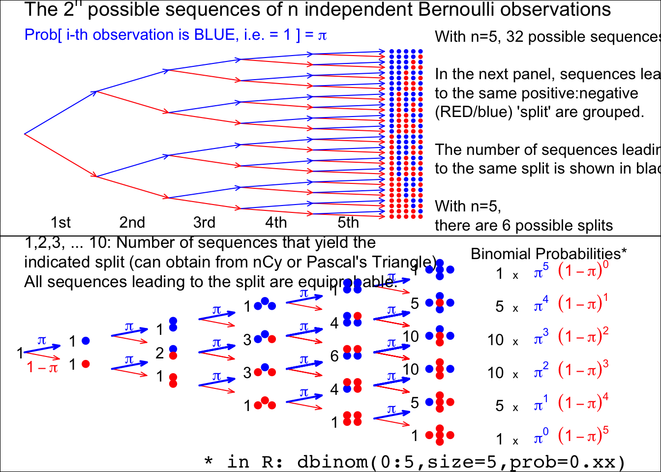
Figure 14.1: From 5 (independent and identically distributed) Bernoulli observations to Binomial(n=5), with the Bernoulli probability left unspecified. There are 2 to the power n possible (distinct) sequences of 0’s and 1’s, each with its probability. We are not interested in these 2 to the power n probabilities, but in the probability that the sample contains y 1’s and (n-y) 0’s. There are only (n+1) possibilities for y, namely 0 to n. Fortunately, each of the n.choose.y sequences that lead to the same sum or count y, has the same probability. So we group the 2.to.power.n sequences into (n+1) sets, according to the sum or count. Each sequence in the set with y 1’s and (n-y) 0’s has the same probability, namely the prob.to.the.power.y times (1-prob).to.the.power.(n-y). Thus, in lieu of adding all such probabilities, we simply multiply this probability by the number, n.choose-y – shown in black – of unique sequences in the set. Check: the frequencies in black add to 2.to.power.n. Nowadays, the (n+1) probabilities are easily obtained by supplying a value for the ‘prob’ argument in the R function dbinom(), instead of computing the binomial coefficient n.choose-y by hand.

If you rotate the binomial tree to the right by 90 degrees, and use your imagination, you can see how it resembles the quincunx constructed by Francis Galton. He used it to show how the Central Linit Theorem, applied to the sum of several ‘Bernoulli deflections to the right and left’, makes a Binomial distribution approach a Gaussian one. Several games and game shows are built on this pinball machine, for example, Plinko and, more recently, The Wall. Galton’s quincunx has its own cottage industry, and versions of it often displayed in Science Museums. The present authors inherited a low tech version of the Galton Board, where the ‘shot’ are turnip seeds, from former McGill Professor – and early teacher of course 607 – FDK Liddell.

14.3.2 Calculating Binomial probabilities

Exactly

• probability mass function (p.m.f.) :

  • formula: \(Prob[y] = \ ^n C _y \ \pi^y \ (1 − \pi)^{n−y}\).

  • recursively: \(Prob[0] = (1−\pi)^n\);    \(Prob[y] = \frac{n−y+1}{y} \times \frac{\pi}{1-\pi} \times Prob[y−1]\).

• Statistical Packages:

  • R functions dbinom(), pbinom(), qbinom()
    probability mass, distribution/cdf, and quantile functions.

  • Stata function Binomial(n,k,p)

  • SAS PROBBNML(p, n, y) function

• Spreadsheet — Excel function BINOMDIST(y, n, π, cumulative)

• Tables: CRC; Fisher and Yates; Biometrika Tables; Documenta Geigy

Using an approximation

• Poisson Distribution (\(n\) large; small \(\pi\))

• Normal (Gaussian) Distribution (\(n\) large or midrange \(\pi\), so that the expected value, \(n \times \pi\), is sufficiently far ‘in from’ the ‘edges’ of the scale, i.e., sufficiently far in from 0 and from \(n\), so that a Gaussian distribution doesn’t flow past one of the edges. The Normal approximation is good for when you don’t have access to software or Tables, e.g, on a plane, or when the internet is down, or the battery on your phone or laptop had run out, or it takes too long to boot up Windows!).
  To use the Normal approximatiom, be aware of the scale you are working in, .e.g., if say \(n = 10\), whether the summary is a count or a proportion or a percentage.

	r.v.	e.g.	E	S.D.
count:	\(y\)	2	\(n \times \pi\)	\(\{n \times \pi \times (1-\pi) \}^{1/2}\)
				i.e., \(n^{1/2} \times \sigma_{Bernoulli}\)
proportion:	\(p=y/n\)	0.2	\(\pi\)	\(\{\pi \times (1-\pi) / n \}^{1/2}\)
				i.e., \(\sigma_{Bernoulli} / n^{1/2}\)
percentage:	\(100p\%\)	20%	\(100 \times \pi\)	\(100 \times SD[p]\)

The first person to suggest an approximation, using what we now call the ‘Normal’ or ‘Gaussian’ of ‘Laplace-Gaussian’ distribution, was deMoivre, in 1738. There is a debate among historians as to whether this marks the first description of the Normal distribution: the piece does not explicitly point to the probability density function \(\frac{1}{\sigma \sqrt{2 \pi}} \times exp[-z^2/2\sigma^2],\) but it does highlight the role of the quantity \((1/2) \times \sqrt{n}\), the standard deviation of the sum of \(n\) independent Bernoulli random variables, each with expectation 1/2 and thus a ‘unit’ standard deviation of 1/2, and also the SD quantity \(\sqrt{\pi(1-\pi)}\) \(\times\) \(\sqrt{n}\) in the more general case. DeMoivre arrived at the familiar ‘68-95-99.7 rule’ : the percentages of a normal distribution that lie within 1, 2 and 3 SD’s of its mean.

Factors that modulate the shapes of Binomial distributions

• size of \(n\): the larger the n, the more symmetric

• value of \(\pi\): the closer to 1/2, the more symmetric

In these small-\(n\) contexts, only those distribtions where \(\pi\) is close to 0.5 are reasonably symmetric.

In larger-\(n\) contexts (see below), as long as there is ‘room’ for them to be, binomial distribtions where the expected value \(E = n \times \pi\) is at least 5-10 ‘in from the edges’ (i.e. to the right of 0, or the left of \(n\), are reasonably symmetric.

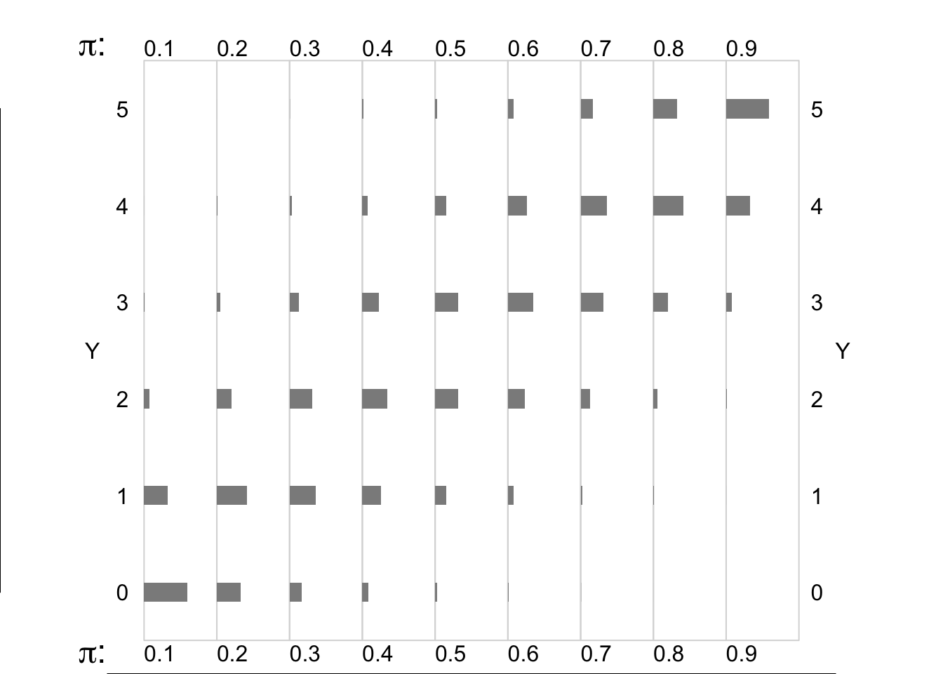
Figure 14.2: Binomial random variables/distributions, where n = 5, and the Bernoulli expectation (probability) is smaller (left panels) or larger (right panels).

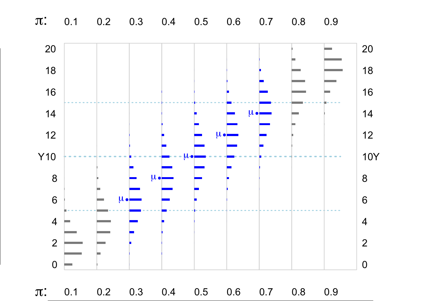
Figure 8.5: Various Binomial random variables/distributions, where n = 20. The dotted horizontal lines in light blue are 5 and 10 units in from the (0,n) boundaries. The distributions where the expected value E or mean, mu ( = n * Bernoulli Probability) is at least 5 units from the (0,n) boundaries are shown in blue.

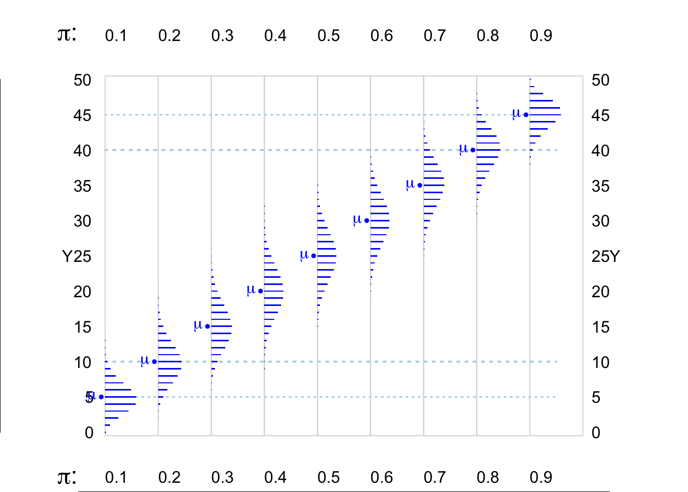
Figure 8.6: Various Binomial random variables/distributions, where n = 50. The blue dotted lines are 5 and 10 units in from the (0,n) boundaries. The distributions where the expected value E or mean, mu ( = n * Bernoulli Probability) is at least 5 units in from the (0,n) boundaries are shown in blue

Back when binomial computations were difficult, and the normal approximation was not accurate, there was another approximation that saved labour, and in particular, avoided having to deal with the very large numbers involved in the \(^nC_y\) binomial coefficients (even if built into a hand calculator, these can be problematic when \(n\) is large).

Poisson, in 1837, having shown how to use the Normal distribution for binomial (and the closely-related negative binomial) calculations, devoted 1 small section (81) of less than 2 pages, to the case where (in our notation) one of the two chances \(\pi\) or \((1-\pi)\) ‘est très petite’ [Poisson’s \(q\) is our \(\pi\), his \(\mu\) is our \(n\), his \(\omega\) is our \(\mu\), and his \(n\) is our \(y\)]. In our notation, he arrived at \[Prob[y \ or \ fewer \ events] = \bigg(1 + \frac{\mu}{1!} + \frac{\mu^2}{2!} + \dots + \frac{\mu^y}{y!} \bigg) \ e^{-\mu}.\]

In the last of his just three paragraphs on this digression, he notes the probability \(e^{-\mu}\) of no event, and \(1 - e^{-\mu}\) of at least 1. He also calculates that, when \(\mu\) = 1, the chance is very close to 1 in 100 million that more than \(y\) = 10 events would occur in a very large series of trials (of length \(n\)), where the probability is 1/\(n\) in each trial. Although he give little emphasis to his formula, and no real application, it is Poisson’s name that is now undividely associated with this formula.

Below are some examples of how well it approximates a Binomial in the ‘corner’ where \(\pi\) is very small and \(n\) is very large. If, of course, the product, \(\mu = n \times \pi\) , reaches double digits, the Normal approximation distribution provides and accurate approximation for both the Binomial and the Poisson distributions, and – if one has ready acccess to the tail areas of a Normal distribution – with less effort. Today, of course, unless you are limited to a hand calculator when the internet and R and paper tables are nor available, you would not need to use any approximation, Normal or Poisson, to a binomial.

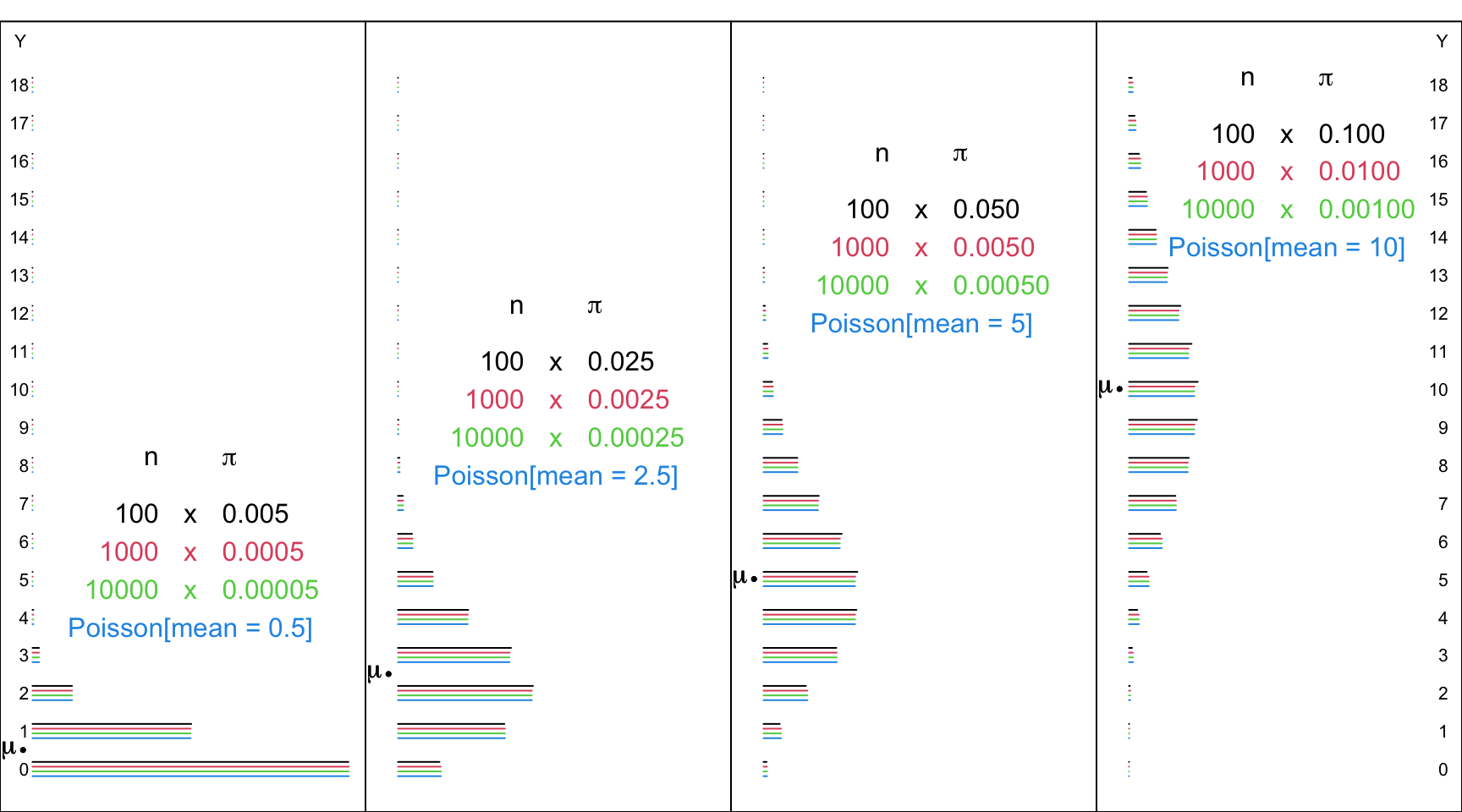
Figure 14.3: Various Binomial random variables/distributions, with large n’s and small Bernoulli probabilities, together with the Poisson distributions with the corresponding means. The Poisson distrubution provides a good approximation in the ’lowee corner of the Bimonial distribution with large n’s and small probabilities. And, when the product, mu = n * probability, is in the double digits, the Normal approximation distribution provides and accurate approximation for both the Binomial and the Poisson distributions.

14.4 When the Binomial does not apply

It does not apply if one (or both) of the ‘i.i.d.’ (independent and identical) conditions do not hold. The first of these conditions is often the one that is absent.

Two very nice examples can be found in Cochran’s (old but still excellent) textbook on sampling. They were re-visited a few decades years ago in connection with what was (then) a new technique for dealing with correlated responses.

The table shows, for each of the 30 randomly sampled households, the number of household members had visited a physician in the previous year. Can we base the precision of the observed proportion, 30/104 or 28%, on a binomial distribution where \(n\) = 104?

True, the ‘n’ in each household is not the same from household to household, but we can segregate the households by size, and carry out separate binomial calculations for each, all the time assuming a common binomial proportion across houdeholds.

XLAB = "y: number in household who has visited an MD in last year"
YLAB = "Number of Households\nfor which y persons visited an MD"

show.household.survey.data(n.who.visited.md,XLAB,YLAB)
#> [1] No. persons with history/trait of interest: 30 / 104 ; Prop'n: 0.29
#> [1]  
#> Below, the row labels are the household sizes.
#> Each column label is the number in a household with history/trait of interest.
#> The entries are how many households had the indicated configuration.
#> 
#>           0    1    2    3    4    5    6    7    Total
#> 1         1    .    .    .    .    .    .    .        1
#> 2         3    .    1    .    .    .    .    .        4
#> 3         7    2    1    2    .    .    .    .       12
#> 4         4    1    3    .    1    .    .    .        9
#> 5         .    .    1    .    .    1    .    .        2
#> 6         1    .    .    .    .    .    .    .        1
#> 7         1    .    .    .    .    .    .    .        1
#> Total    17    3    6    2    1    1    0    0       30
#> 
#> Same row/col meanings, but theoretical, binomial-based,
#> EXPECTED frequencies of households having these many persons
#>  who would have -- if all 128 persons were independently sampled
#> from a population where the proportion with 
#> the history/trait of interest was as above.
#> 
#>           0     1     2     3     4     5     6     7 Total
#> 1     0.712 0.288     .     .     .     .     .     .     1
#> 2     1.013 0.821 0.166     .     .     .     .     .     4
#> 3     1.081 1.314 0.533 0.072     .     .     .     .    12
#> 4     1.025 1.663 1.011 0.273 0.028     .     .     .     9
#> 5     0.912 1.849 1.499 0.608 0.123 0.010     .     .     2
#> 6     0.779 1.894 1.920 1.038 0.315 0.051 0.003     .     1
#> 7     0.646 1.834 2.231 1.507 0.611 0.149 0.020 0.001     1
#> Total 6.167 9.663 7.360 3.498 1.077 0.210 0.024 0.001    30
#> 
#> We will just assess the fit on the 'totals'row:
#>  the numbers in the individual rows are too small to judge.
#> 
#>         0   1   2   3   4   5 6 7 Total
#> [1,] 17.0 3.0 6.0 2.0 1.0 1.0 0 0    30
#> [2,]  6.2 9.7 7.4 3.5 1.1 0.2 0 0    30
#> 
#> Better still, here is a picture: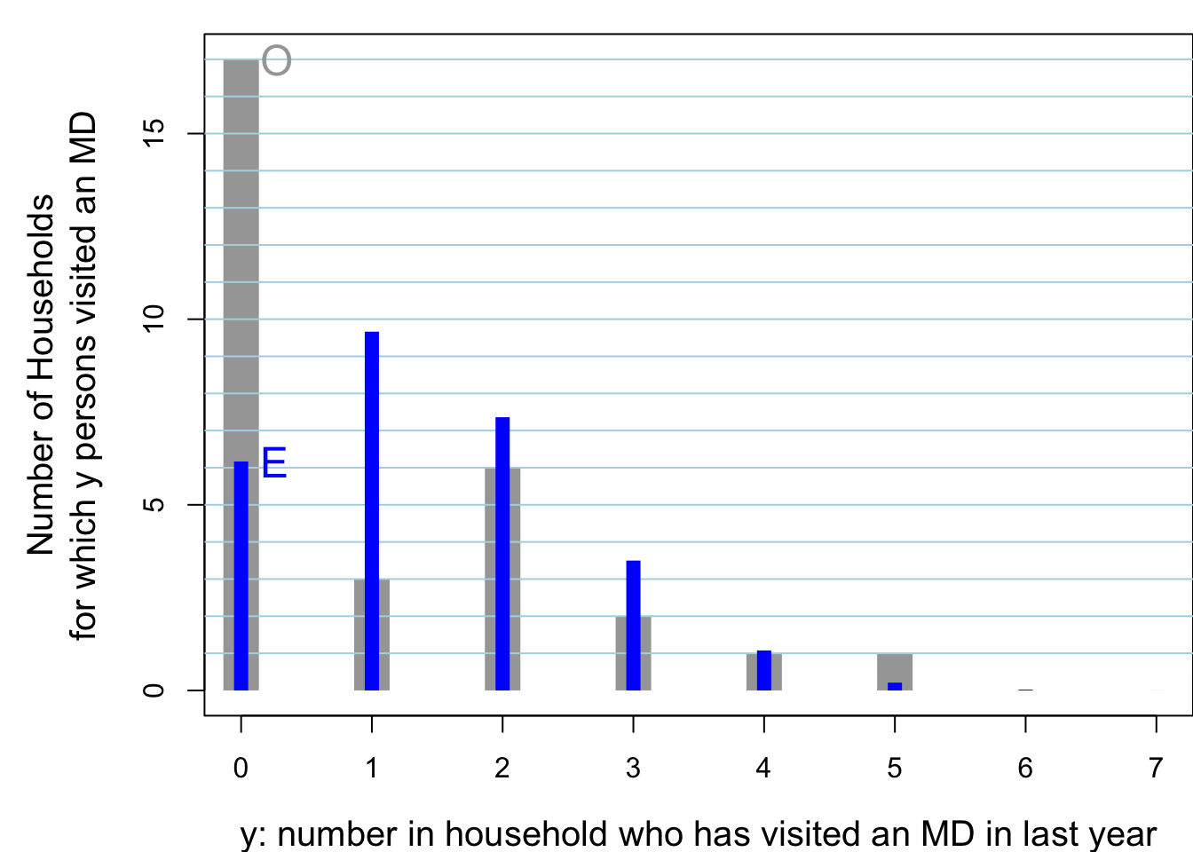

Figure 14.4: Of 30 randomly sampled households, (O)bserved numbers of households, shown in grey, where 0, 1, .. in household had visited a physician in the previous year. The 30 households contained 104 persons, 28 of whom had visited a physician in the previous year. Also shown, in blue are the (E)xpected numbers of households, assuming the data were generated from 104 independent Bernoulli random variables, each with the same probability 28/104. The observed variance is considerably LARGER than that predicted by a binomial distribution. You would see this even if the individuals in the house were not from the same family. For example, if the occupants were students, the proportion of them with such a history would be different (?lower) than if the occupants were older: this is the ‘non-identical probabilities’ aspect. The other possibility, the ‘non-independence’ aspect, is that health status and the seeking medical care are affected by shared family factors, such as behaviours, attitudes, lifestyle, and insurance coverage.

Cochran provides this explanation for the greater than binomial variation in the proportions

The variance given by the ratio method, 0.00520, is much larger than that given by the binomial formula, 0.00197. For various reasons, families differ in the frequency with which their members consult a doctor. For the sample as a whole, the proportion who consult a doctor is only a little more than one in four, but there are several families in which every member has seen a doctor. Similar results would be obtained for any characteristic in which the members of the same family tend to act in the same way.

Clearly, if we are dealing with an infectious disease, we would need to be very careful about our statistical model for the numbers in a family or household or care facility that are affected.

XLAB = "y: number of males in household"
YLAB=  "Number of Households\n where y persons were male"
show.household.survey.data(n.males,XLAB,YLAB)
#> [1] No. persons with history/trait of interest: 53 / 104 ; Prop'n: 0.51
#> [1]  
#> Below, the row labels are the household sizes.
#> Each column label is the number in a household with history/trait of interest.
#> The entries are how many households had the indicated configuration.
#> 
#>          0     1    2    3    4    5    6    7    Total
#> 1        1     .    .    .    .    .    .    .        1
#> 2        .     4    .    .    .    .    .    .        4
#> 3        .     7    5    .    .    .    .    .       12
#> 4        .     1    3    5    .    .    .    .        9
#> 5        .     1    .    1    .    .    .    .        2
#> 6        .     .    .    1    .    .    .    .        1
#> 7        .     .    .    1    .    .    .    .        1
#> Total    1    13    8    8    0    0    0    0       30
#> 
#> Same row/col meanings, but theoretical, binomial-based,
#> EXPECTED frequencies of households having these many persons
#>  who would have -- if all 128 persons were independently sampled
#> from a population where the proportion with 
#> the history/trait of interest was as above.
#> 
#>           0     1     2     3     4     5     6     7 Total
#> 1     0.490 0.510     .     .     .     .     .     .     1
#> 2     0.481 1.000 0.519     .     .     .     .     .     4
#> 3     0.354 1.103 1.146 0.397     .     .     .     .    12
#> 4     0.231 0.962 1.499 1.038 0.270     .     .     .     9
#> 5     0.142 0.737 1.531 1.591 0.827 0.172     .     .     2
#> 6     0.083 0.520 1.352 1.873 1.460 0.607 0.105     .     1
#> 7     0.048 0.347 1.083 1.875 1.949 1.215 0.421 0.062     1
#> Total 1.829 5.178 7.130 6.775 4.505 1.994 0.526 0.062    30
#> 
#> We will just assess the fit on the 'totals'row:
#>  the numbers in the individual rows are too small to judge.
#> 
#>        0    1   2   3   4 5   6   7 Total
#> [1,] 1.0 13.0 8.0 8.0 0.0 0 0.0 0.0    30
#> [2,] 1.8  5.2 7.1 6.8 4.5 2 0.5 0.1    30
#> 
#> Better still, here is a picture: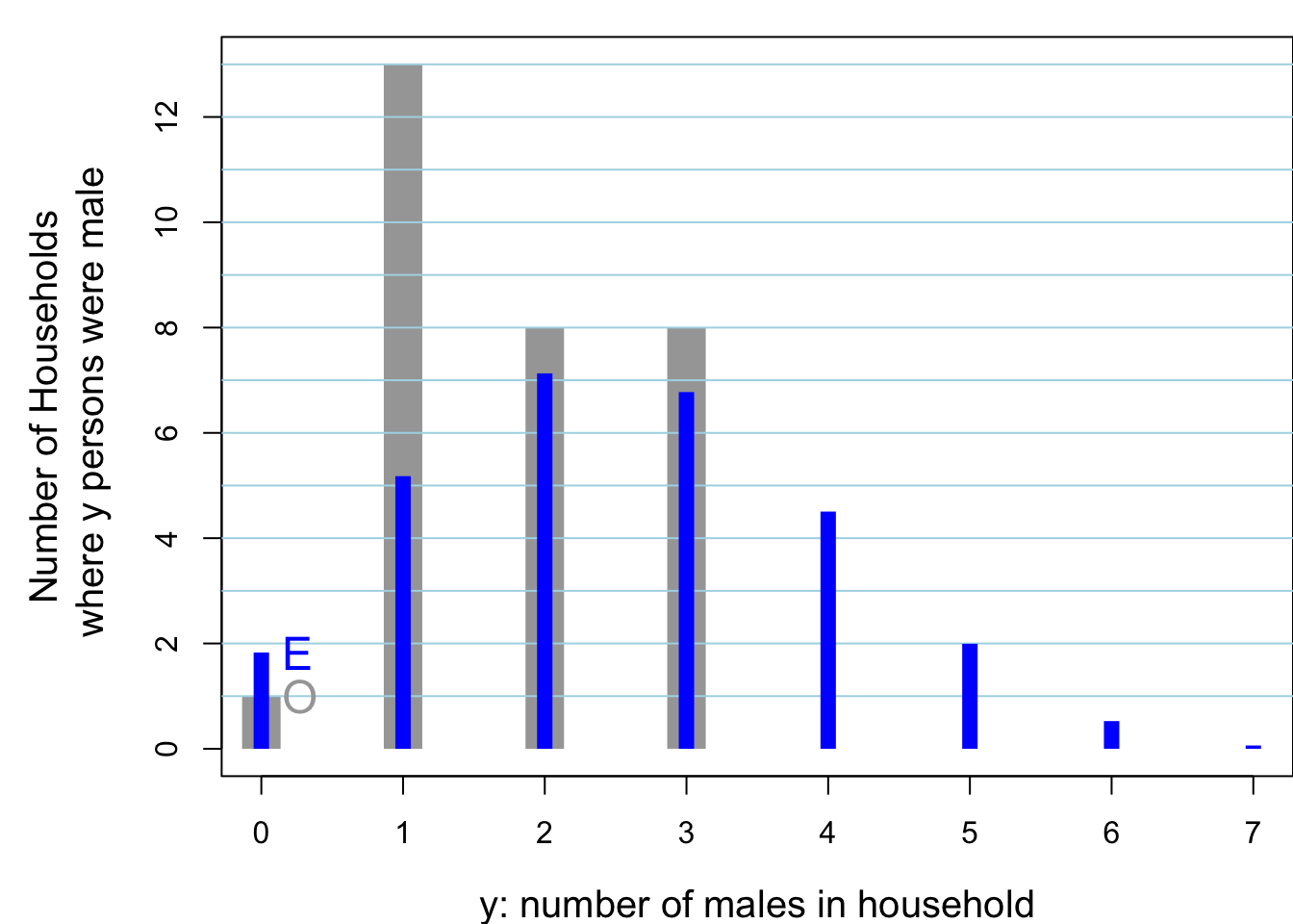

Figure 8.9: Of 30 randomly sampled households, (O)bserved numbers of households, shown in grey, where 0, 1, .. in household were male. The 30 households contained 104 persons, 53 of whom were male. Also shown, in blue are the (E)xpected numbers of households, assuming the data were generated from 104 independent Bernoulli random variables, each with the same probability 53/104. The observed variance is considerably SMALLER than that predicted by a binomial distribution. You would see this even if the individuals in the house were not from the same family. For example, if the occupants were students, the proportion of them with such a history would be different (?lower) than if the occupants were older: this is the ‘non-identical probabilities’ aspect. The other possibility, the ‘non-independence’ aspect, is that health status and the seeking medical care are affected by shared family factors, such as behaviours, attitudes, lifestyle, and insurance coverage.

Cochran provides this explanation for the (unsually) less than binomial variation seen in this response variable.

In estimating the proportion of males in the population, the results are different. By the same type of calculation, we find binomial formula: v(p) = 0.00240; ratio formula v(p) = 0.00114
Here the binomial formula overestimates the variance. The reason is interesting. Most households are set up as a result of a marriage, hence contain at least one male and one female. Consequently the proportion of males per family varies less from one half than would be expected from the binomial formula. None of the 30 families, except one with only one member, is composed entirely of males, or entirely of females. If the binomial distribution were applicable, with a true P of approximately one half, households with all members of the same sex would constitute one quarter of the households of size 3 and one eighth of the households of size 4. This property of the sex ratio has been discussed by Hansen and Hurwitz (1942). Other illustrations of the error committed by improper use of the binomial formula in sociological investigations have been given by Kish (1957).

Does the Binomial Distribution apply if… ?

Interested in:	\(\pi\)	the proportion of 16 year old girls in Quebec protected against rubella
Choose:	\(n\) = 100	girls: 20 at random from each of 5 randomly selected schools [‘cluster’ sample]
Count	\(y\)	how many of the \(n\) = 100 are protected
		\(\bullet\) Is \(y ~ \sim Binomial(n=100, \ \pi)\) ?
………….	………..	………………………………………………………
‘SMAC’:	\(\pi\)	Chemistry Auto-analyzer with n = 18 channels. Critertion for ‘positivity’ set so that Prob[‘abnormal’ result in Healthy person] = 0.03 for each of 18 chemistries tested
Count	\(y\)	(In 1 patient) how many of \(n\) = 18 give abnormal result.
		\(\bullet\) Is \(y ~ \sim Binomial(n=18, \ \pi=0.03)\) ? credit: Ingelfinger textbook
………….	………..	………………………………………………………
………….	………..	………………………………………………………
Sex Ratio:	\(n=4\)	children in each family
	\(y\)	number of girls in family
		\(\bullet\) Is \(y ~ \sim Binomial(n=4, \ \pi=0.49)\) ?
………….	………..	………………………………………………………
Interested in:	\(\pi_u\)	proportion in ‘usual’ exercise classes and in
	\(\pi_e\)	expt’l. exercise classes who ‘stay the course’
Randomly	4	classes of
Allocate	25	students each to usual course
	\(n_u = 4 \times 25 = 100\)
	\(n_e\) = 4	classes of
	25	students each to experimental course
	\(n_e = 4 \times 25 =100\)
Count	\(y_u\)	how many of the \(n_u\) = 100 complete course
	\(y_e\)	how many of the \(n_e\) = 100 complete course
		\(\bullet\) Is \(y_u ~ \sim Binomial(n = 100, \ \pi_u)\) ?
		\(\bullet\) Is \(y_e ~ \sim Binomial(n = 100, \ \pi_e)\) ?
………….	………..	………………………………………………………
Pilot Study:		To estimate proportion \(\pi\) of population that is eligible and willing to participate in long-term research study, keep recruiting until obtain
	\(y\) = 5	who are. Have to approach \(n\) to get \(y\).
		\(\bullet\) Is \(y ~ \sim Binomial(n, \ \pi)\) ?
………….	………..	………………………………………………………

14.5 More on the Approximation of the Binomial Distribution

The Normal distribution emerges frequently as an approximation of the distribution of data characteristics. The probability theory that mathematically establishes such approximation is called the Central Limit Theorem. In this section we demonstrate the Normal approximation in the context of the Binomial distribution.

14.5.1 Approximate Binomial Probabilities and Percentiles

Consider, for example, the probability of obtaining between 1940 and 2060 heads when tossing 4,000 fair coins. Let \(Y\) be the total number of heads. The tossing of a coin is a trial with two possible outcomes: “Head” and “Tail.” The probability of a “Head” is 0.5 and there are 4,000 trials. Let us call obtaining a “Head” in a trial a “Success”. Observe that the random variable \(Y\) counts the total number of successes. Hence, \(Y \sim \mathrm{Binomial}(4000,0.5)\).

The probability \(\operatorname{P}(1940 \leq Y \leq 2060)\) can be computed as the difference between the probability \(\operatorname{P}(Y \leq 2060)\) of being less or equal to 2060 and the probability \(\operatorname{P}(Y < 1940)\) of being strictly less than 1940. However, 1939 is the largest integer that is still strictly less than the integer 1940. As a result we get that \(\operatorname{P}(Y < 1940) = \operatorname{P}(Y \leq 1939)\). Consequently, \(\operatorname{P}(1940 \leq Y \leq 2060) = \operatorname{P}(Y \leq 2060) - \operatorname{P}(Y \leq 1939)\).

Applying the function “pbinom” for the computation of the Binomial cumulative probability, namely the probability of being less or equal to a given value, we get that the probability in the range between 1940 and 2060 is equal to

pbinom(2060,4000,0.5) - pbinom(1939,4000,0.5)
#> [1] 0.9442883

This is an exact computation. The Normal approximation produces an approximate evaluation, not an exact computation. The Normal approximation replaces Binomial computations by computations carried out for the Normal distribution. The computation of a probability for a Binomial random variable is replaced by computation of probability for a Normal random variable that has the same expectation and standard deviation as the Binomial random variable.

Notice that if \(Y \sim \mathrm{Binomial}(4000,0.5)\) then the expectation is \(\operatorname{E}(Y) = 4,000 \times 0.5 = 2,000\) and the variance is \(\operatorname{Var}(Y) = 4,000 \times 0.5 \times 0.5 = 1,000\), with the standard deviation being the square root of the variance. Repeating the same computation that we conducted for the Binomial random variable, but this time with the function “pnorm” that is used for the computation of the Normal cumulative probability, we get:

mu <- 4000*0.5
sig <- sqrt(4000*0.5*0.5)
pnorm(2060,mu,sig) - pnorm(1939,mu,sig)
#> [1] 0.9442441

Observe that in this example the Normal approximation of the probability (0.9442441) agrees with the Binomial computation of the probability (0.9442883) up to 3 significant digits.

Normal computations may also be applied in order to find approximate percentiles of the Binomial distribution. For example, let us identify the central region that contains for a \(\mathrm{Binomial}(4000,0.5)\) random variable (approximately) 95% of the distribution. Towards that end we can identify the boundaries of the region for the Normal distribution with the same expectation and standard deviation as that of the target Binomial distribution:

qnorm(0.975,mu,sig)
#> [1] 2061.98
qnorm(0.025,mu,sig)
#> [1] 1938.02

After rounding to the nearest integer we get the interval \([1938,2062]\) as a proposed central region.

In order to validate the proposed region we may repeat the computation under the actual Binomial distribution:

qbinom(0.975,4000,0.5)
#> [1] 2062
qbinom(0.025,4000,0.5)
#> [1] 1938

Again, we get the interval \([1938,2062]\) as the central region, in agreement with the one proposed by the Normal approximation. Notice that the function “qbinom” produces the percentiles of the Binomial distribution.

The ability to approximate one distribution by the other, when computation tools for both distributions are handy, seems to be of questionable importance. Indeed, the significance of the Normal approximation is not so much in its ability to approximate the Binomial distribution as such. Rather, the important point is that the Normal distribution may serve as an approximation to a wide class of distributions, with the Binomial distribution being only one example. Computations that are based on the Normal approximation will be valid for all members in the class of distributions, including cases where we don’t have the computational tools at our disposal or even in cases where we do not know what the exact distribution of the member is (aka the CLT).

On the other hand, one need not assume that any distribution is well approximated by the Normal distribution. For example, the distribution of wealth in the population tends to be skewed, with more than 50% of the people possessing less than 50% of the wealth and small percentage of the people possessing the majority of the wealth. The Normal distribution is not a good model for such distribution. The Exponential distribution, or distributions similar to it, may be more appropriate.

14.5.2 Continuity Corrections

In order to complete this section let us look more carefully at the Normal approximations of the Binomial distribution.

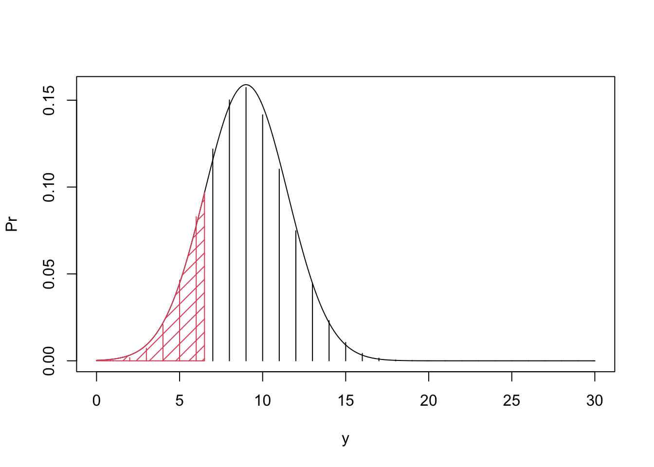
Figure 9.7: Normal Approximation of the Binomial Distribution

In principle, the Normal approximation is valid when \(n\), the number of independent trials in the Binomial distribution, is large. When \(n\) is relatively small the approximation may not be so good. Indeed, take \(Y \sim \mathrm{Binomial}(30,0.3)\) and consider the probability \(\operatorname{P}(Y \leq 6)\). Compare the actual probability to the Normal approximation:

pbinom(6,30,0.3)
#> [1] 0.159523
pnorm(6,30*0.3,sqrt(30*0.3*0.7))
#> [1] 0.1159989

The Normal approximation, which is equal to 0.1159989, is not too close to the actual probability, which is equal to 0.1595230.

A naïve application of the Normal approximation for the \(\mathrm{Binomial}(n,p)\) distribution may not be so good when the number of trials \(n\) is small. Yet, a small modification of the approximation may produce much better results. In order to explain the modification consult Figure 9.7 where you will find the bar plot of the Binomial distribution with the density of the approximating Normal distribution superimposed on top of it. The target probability is the sum of heights of the bars that are painted in red. In the naïve application of the Normal approximation we used the area under the normal density which is to the left of the bar associated with the value \(y=6\).

Alternatively, you may associate with each bar located at \(y\) the area under the normal density over the interval \([y-0.5, y+0.5]\). The resulting correction to the approximation will use the Normal probability of the event \(\{Y \leq 6.5\}\), which is the area shaded in red. The application of this approximation, which is called continuity correction produces:

pnorm(6.5,30*0.3,sqrt(30*0.3*0.7))
#> [1] 0.1596193

Observe that the corrected approximation is much closer to the target probability, which is 0.1595230, and is substantially better that the uncorrected approximation which was 0.1159989. Generally, it is recommended to apply the continuity correction to the Normal approximation of a discrete distribution.

Consider the \(\mathrm{Binomial}(n,p)\) distribution. Another situation where the Normal approximation may fail is when \(p\), the probability of “Success” in the Binomial distribution, is too close to 0 (or too close to 1).

14.6 Exercises

A particular measles vaccine produces a reaction (a fever higher that 102 Fahrenheit) in each vaccinee with probability of 0.09. A clinic vaccinates 500 people each day.

1. What is the expected number of people that will develop a reaction each day?

2. What is the standard deviation of the number of people that will develop a reaction each day?

3. In a given day, what is the probability that more than 40 people will develop a reaction?

4. In a given day, what is the probability that the number of people that will develop a reaction is between 50 and 45 (inclusive)?

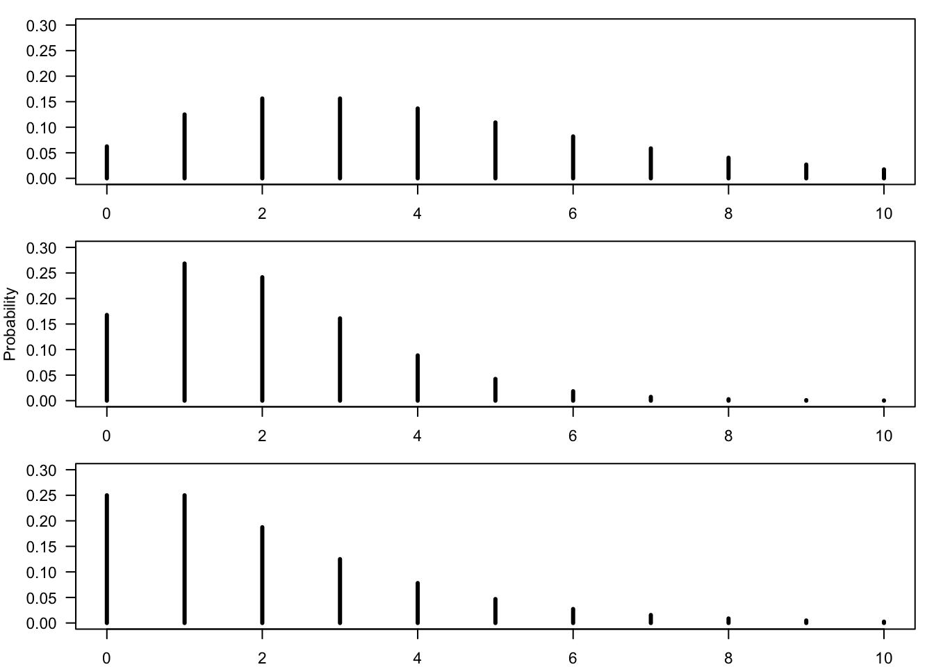
Figure 14.5: Bar Plots of the Negative-Binomial Distribution

14.7 Summary

Glossary

Binomial Random Variable:

The number of successes among \(n\) repeats of independent trials with a probability \(p\) of success in each trial. The distribution is marked as \(\mathrm{Binomial}(n,p)\).

Density:

Histogram that describes the distribution of a continuous random variable. The area under the curve corresponds to probability.

Summary of Formulas

Discrete Random Variable:

\[\begin{aligned} \operatorname{E}(Y) &= \sum_y \big(y \times \operatorname{P}(y)\big) \\ \operatorname{Var}(Y) &= \sum_y\big( (y-\operatorname{E}(Y))^2 \times \operatorname{P}(y)\big) \end{aligned}\]

Binomial:

\(\operatorname{E}(Y) = n p \;, \quad \operatorname{Var}(Y) = n p(1-p)\)